Chapter 1 RHC data description
There is a widespread belief among cardiologists that the right heart catheterization (RHC hereafter; a monitoring device for measurement of cardiac function) is helpful in managing critically ill patients in the intensive care unit. Connors et al. (1996) examined the association of
- RHC use during the first 24 hours of care in the intensive care unit and
- a number of health-outcomes such as length of stay (hospital).
1.1 Data download
# load the dataset
ObsData <- read.csv("https://hbiostat.org/data/repo/rhc.csv", header = TRUE)
saveRDS(ObsData, file = "data/rhc.RDS")
1.2 Analytic data
Below we show the process of creating the analytic data (optional).
# add column for outcome Y: length of stay
# Y = date of discharge - study admission date
# Y = date of death - study admission date if date of discharge not available
ObsData$Y <- ObsData$dschdte - ObsData$sadmdte
ObsData$Y[is.na(ObsData$Y)] <- ObsData$dthdte[is.na(ObsData$Y)] -
  ObsData$sadmdte[is.na(ObsData$Y)]
# remove outcomes we are not examining in this example
ObsData <- dplyr::select(ObsData,
                         !c(dthdte, lstctdte, dschdte, death, t3d30, dth30, surv2md1))
# remove unnecessary and problematic variables
ObsData <- dplyr::select(ObsData,
                         !c(sadmdte, ptid, X, adld3p, urin1, cat2))

# convert all categorical variables to factors
factors <- c("cat1", "ca", "cardiohx", "chfhx", "dementhx", "psychhx",
             "chrpulhx", "renalhx", "liverhx", "gibledhx", "malighx",
             "immunhx", "transhx", "amihx", "sex", "dnr1", "ninsclas",
             "resp", "card", "neuro", "gastr", "renal", "meta", "hema",
             "seps", "trauma", "ortho", "race", "income")
ObsData[factors] <- lapply(ObsData[factors], as.factor)
# convert our treatment A (RHC vs. No RHC) to a binary variable
ObsData$A <- ifelse(ObsData$swang1 == "RHC", 1, 0)
ObsData <- dplyr::select(ObsData, !swang1)
# Categorize the variables to match with the original paper
ObsData$age <- cut(ObsData$age,breaks=c(-Inf, 50, 60, 70, 80, Inf),right=FALSE)
ObsData$race <- factor(ObsData$race, levels=c("white","black","other"))
ObsData$sex <- as.factor(ObsData$sex)
ObsData$sex <- relevel(ObsData$sex, ref = "Male")
ObsData$cat1 <- as.factor(ObsData$cat1)
levels(ObsData$cat1) <- c("ARF","CHF","Other","Other","Other",
                          "Other","Other","MOSF","MOSF")
ObsData$ca <- as.factor(ObsData$ca)
levels(ObsData$ca) <- c("Metastatic","None","Localized (Yes)")
ObsData$ca <- factor(ObsData$ca, levels=c("None",
                                          "Localized (Yes)","Metastatic"))
# Rename variables
names(ObsData) <- c("Disease.category", "Cancer", "Cardiovascular",
                    "Congestive.HF", "Dementia", "Psychiatric", "Pulmonary",
                    "Renal", "Hepatic", "GI.Bleed", "Tumor",
                    "Immunosupperssion", "Transfer.hx", "MI", "age", "sex",
                    "edu", "DASIndex", "APACHE.score", "Glasgow.Coma.Score",
                    "blood.pressure", "WBC", "Heart.rate", "Respiratory.rate",
                    "Temperature", "PaO2vs.FIO2", "Albumin", "Hematocrit",
                    "Bilirubin", "Creatinine", "Sodium", "Potassium", "PaCo2",
                    "PH", "Weight", "DNR.status", "Medical.insurance",
                    "Respiratory.Diag", "Cardiovascular.Diag",
                    "Neurological.Diag", "Gastrointestinal.Diag", "Renal.Diag",
                    "Metabolic.Diag", "Hematologic.Diag", "Sepsis.Diag",
                    "Trauma.Diag", "Orthopedic.Diag", "race", "income",
                    "Y", "A")
saveRDS(ObsData, file = "data/rhcAnalytic.RDS")
1.3 Notations
| Notations | Example in RHC study |
|---|---|
| \(A\): Exposure status | RHC |
| \(Y\): Observed outcome | length of stay |
| \(L\): Covariates | See below |
1.4 Variables
baselinevars <- names(dplyr::select(ObsData,
                         !c(A,Y)))
baselinevars
## [1] "Disease.category" "Cancer" "Cardiovascular"
## [4] "Congestive.HF" "Dementia" "Psychiatric"
## [7] "Pulmonary" "Renal" "Hepatic"
## [10] "GI.Bleed" "Tumor" "Immunosupperssion"
## [13] "Transfer.hx" "MI" "age"
## [16] "sex" "edu" "DASIndex"
## [19] "APACHE.score" "Glasgow.Coma.Score" "blood.pressure"
## [22] "WBC" "Heart.rate" "Respiratory.rate"
## [25] "Temperature" "PaO2vs.FIO2" "Albumin"
## [28] "Hematocrit" "Bilirubin" "Creatinine"
## [31] "Sodium" "Potassium" "PaCo2"
## [34] "PH" "Weight" "DNR.status"
## [37] "Medical.insurance" "Respiratory.Diag" "Cardiovascular.Diag"
## [40] "Neurological.Diag" "Gastrointestinal.Diag" "Renal.Diag"
## [43] "Metabolic.Diag" "Hematologic.Diag" "Sepsis.Diag"
## [46] "Trauma.Diag" "Orthopedic.Diag" "race"
## [49] "income"1.5 Table 1 stratified by RHC exposure
Only for some demographic and co-morbidity variables; match with Table 1 in Connors et al. (1996).
require(tableone)
tab0 <- CreateTableOne(vars = c("age", "sex", "race", "Disease.category", "Cancer"),
                       data = ObsData,
                       strata = "A",
                       test = FALSE)
print(tab0, showAllLevels = FALSE, )
## Stratified by A
## 0 1
## n 3551 2184
## age (%)
## [-Inf,50) 884 (24.9) 540 (24.7)
## [50,60) 546 (15.4) 371 (17.0)
## [60,70) 812 (22.9) 577 (26.4)
## [70,80) 809 (22.8) 529 (24.2)
## [80, Inf) 500 (14.1) 167 ( 7.6)
## sex = Female (%) 1637 (46.1) 906 (41.5)
## race (%)
## white 2753 (77.5) 1707 (78.2)
## black 585 (16.5) 335 (15.3)
## other 213 ( 6.0) 142 ( 6.5)
## Disease.category (%)
## ARF 1581 (44.5) 909 (41.6)
## CHF 247 ( 7.0) 209 ( 9.6)
## Other 955 (26.9) 208 ( 9.5)
## MOSF 768 (21.6) 858 (39.3)
## Cancer (%)
## None 2652 (74.7) 1727 (79.1)
## Localized (Yes) 638 (18.0) 334 (15.3)
## Metastatic 261 ( 7.4) 123 ( 5.6)Only outcome variable (Length of stay); slightly different than Table 2 in Connors et al. (1996) (means 20.5 vs. 25.7; and medians 13 vs. 17).
tab1 <- CreateTableOne(vars = c("Y"),
                       data = ObsData,
                       strata = "A",
                       test = FALSE)
print(tab1, showAllLevels = FALSE, )
## Stratified by A
## 0 1
## n 3551 2184
## Y (mean (SD)) 19.53 (23.59) 24.86 (28.90)median(ObsData$Y[ObsData$A==0]); median(ObsData$Y[ObsData$A==1])## [1] 12## [1] 161.6 Basic regression analysis
1.6.1 Crude analysis
# adjust the exposure variable (primary interest)
fit0 <- lm(Y~A, data = ObsData)
require(Publish)
crude.fit <- publish(fit0, digits=1)$regressionTable[2,]crude.fit## Variable Units Coefficient CI.95 p-value
## 2 A 5.3 [4.0;6.7] <0.11.6.2 Adjusted analysis
# adjust the exposure variable (primary interest) + covariates
out.formula <- as.formula(paste("Y~ A +",
                               paste(baselinevars,
                                     collapse = "+")))
fit1 <- lm(out.formula, data = ObsData)
adj.fit <- publish(fit1, digits=1)$regressionTable[2,]saveRDS(fit1, file = "data/adjreg.RDS")out.formula## Y ~ A + Disease.category + Cancer + Cardiovascular + Congestive.HF +
## Dementia + Psychiatric + Pulmonary + Renal + Hepatic + GI.Bleed +
## Tumor + Immunosupperssion + Transfer.hx + MI + age + sex +
## edu + DASIndex + APACHE.score + Glasgow.Coma.Score + blood.pressure +
## WBC + Heart.rate + Respiratory.rate + Temperature + PaO2vs.FIO2 +
## Albumin + Hematocrit + Bilirubin + Creatinine + Sodium +
## Potassium + PaCo2 + PH + Weight + DNR.status + Medical.insurance +
## Respiratory.Diag + Cardiovascular.Diag + Neurological.Diag +
## Gastrointestinal.Diag + Renal.Diag + Metabolic.Diag + Hematologic.Diag +
## Sepsis.Diag + Trauma.Diag + Orthopedic.Diag + race + incomeadj.fit| Variable | Units | Coefficient | CI.95 | p-value |
|---|---|---|---|---|
| A | 2.9 | [1.4;4.4] | <0.1 |
1.6.3 Regression diagnostics
plot(fit1)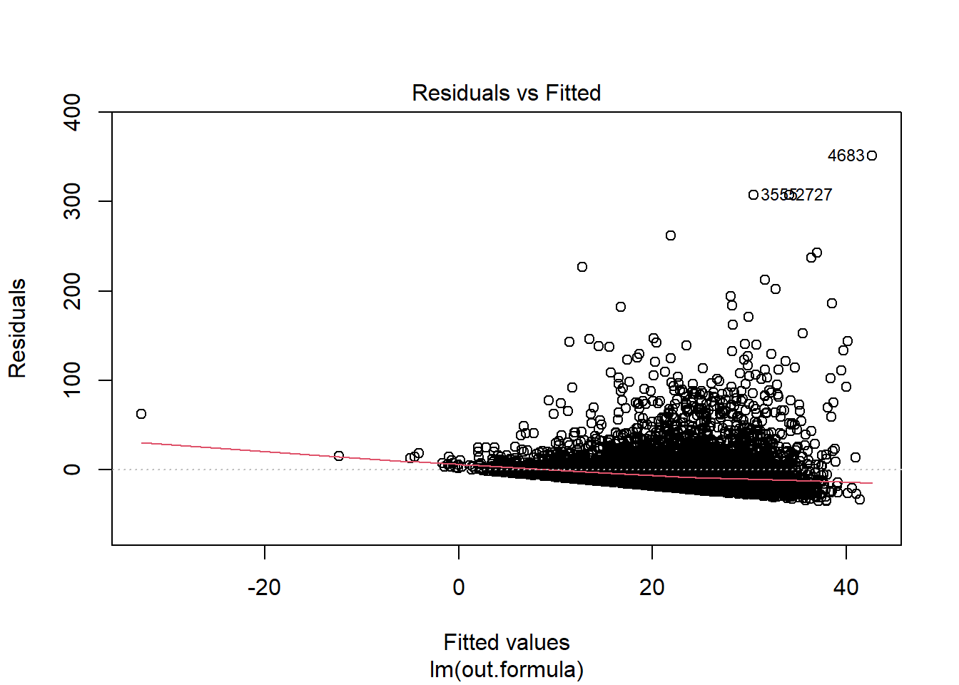
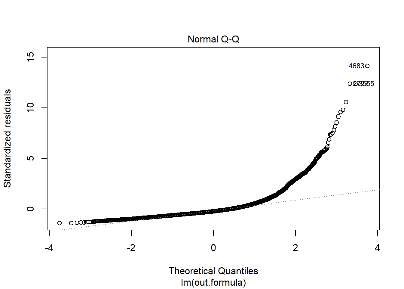
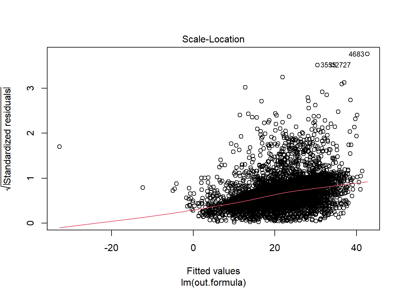
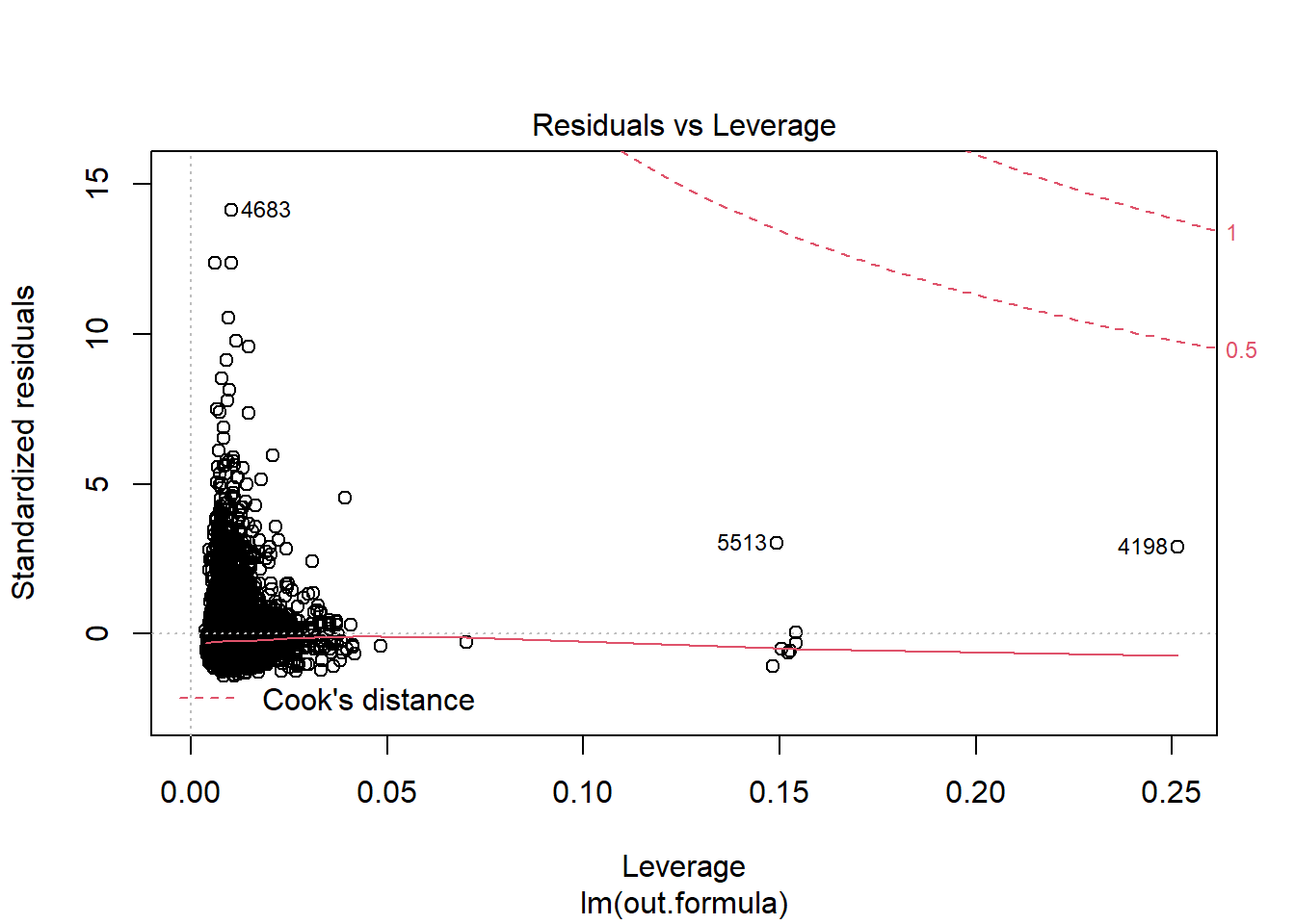
Diagnostics do not necessarily look so good.
1.7 Comparison with literature
Connors et al. (1996) conducted a propensity score matching analysis.
Table 5 in Connors et al. (1996) showed that, after propensity score pair (1-to-1) matching, means of length of stay (\(Y\)), when stratified by RHC (\(A\)) were not significantly different (\(p = 0.14\)).
1.7.1 PSM in RHC data
We also conduct propensity score pair matching analysis, as follows.
Note: In this workshop, we will not cover Propensity Score Matching (PSM). If you want to learn more about this, feel free to check out this other workshop: Understanding Propensity Score Matching and the video recording on youtube.
set.seed(111)
require(MatchIt)
ps.formula <- as.formula(paste("A~",
                paste(baselinevars, collapse = "+")))
PS.fit <- glm(ps.formula,family="binomial",
              data=ObsData)
ObsData$PS <- predict(PS.fit,
                      newdata = ObsData, type="response")
logitPS <- -log(1/ObsData$PS - 1)
match.obj <- matchit(ps.formula, data =ObsData,
distance = ObsData$PS,
method = "nearest", replace=FALSE,
ratio = 1,
caliper = .2*sd(logitPS))1.7.1.1 PSM diagnostics
require(cobalt)
bal.plot(match.obj,
         var.name = "distance",
         which = "both",
         type = "histogram",
         mirror = TRUE)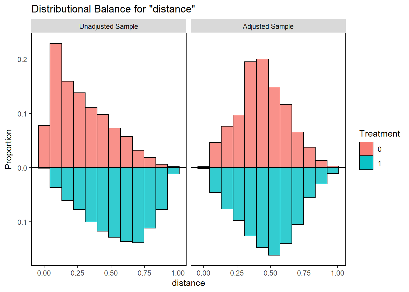
bal.tab(match.obj, un = TRUE,
        thresholds = c(m = .1))
## Call
## matchit(formula = ps.formula, data = ObsData, method = "nearest",
## distance = ObsData$PS, replace = FALSE, caliper = 0.2 * sd(logitPS),
## ratio = 1)
##
## Balance Measures
## Type Diff.Un Diff.Adj M.Threshold
## distance Distance 1.1558 0.1820
## Disease.category_ARF Binary -0.0290 -0.0178 Balanced, <0.1
## Disease.category_CHF Binary 0.0261 -0.0006 Balanced, <0.1
## Disease.category_Other Binary -0.1737 -0.0092 Balanced, <0.1
## Disease.category_MOSF Binary 0.1766 0.0276 Balanced, <0.1
## Cancer_None Binary 0.0439 0.0075 Balanced, <0.1
## Cancer_Localized (Yes) Binary -0.0267 -0.0109 Balanced, <0.1
## Cancer_Metastatic Binary -0.0172 0.0035 Balanced, <0.1
## Cardiovascular Binary 0.0445 -0.0104 Balanced, <0.1
## Congestive.HF Binary 0.0268 0.0012 Balanced, <0.1
## Dementia Binary -0.0472 -0.0023 Balanced, <0.1
## Psychiatric Binary -0.0348 -0.0081 Balanced, <0.1
## Pulmonary Binary -0.0737 -0.0138 Balanced, <0.1
## Renal Binary 0.0066 -0.0058 Balanced, <0.1
## Hepatic Binary -0.0124 -0.0023 Balanced, <0.1
## GI.Bleed Binary -0.0122 -0.0006 Balanced, <0.1
## Tumor Binary -0.0423 -0.0052 Balanced, <0.1
## Immunosupperssion Binary 0.0358 -0.0046 Balanced, <0.1
## Transfer.hx Binary 0.0554 0.0115 Balanced, <0.1
## MI Binary 0.0139 -0.0012 Balanced, <0.1
## age_[-Inf,50) Binary -0.0017 0.0063 Balanced, <0.1
## age_[50,60) Binary 0.0161 0.0104 Balanced, <0.1
## age_[60,70) Binary 0.0355 0.0006 Balanced, <0.1
## age_[70,80) Binary 0.0144 -0.0132 Balanced, <0.1
## age_[80, Inf) Binary -0.0643 -0.0040 Balanced, <0.1
## sex_Female Binary -0.0462 -0.0092 Balanced, <0.1
## edu Contin. 0.0910 0.0293 Balanced, <0.1
## DASIndex Contin. 0.0654 0.0263 Balanced, <0.1
## APACHE.score Contin. 0.4837 0.0813 Balanced, <0.1
## Glasgow.Coma.Score Contin. -0.1160 -0.0147 Balanced, <0.1
## blood.pressure Contin. -0.4869 -0.0680 Balanced, <0.1
## WBC Contin. 0.0799 -0.0096 Balanced, <0.1
## Heart.rate Contin. 0.1460 -0.0005 Balanced, <0.1
## Respiratory.rate Contin. -0.1641 -0.0361 Balanced, <0.1
## Temperature Contin. -0.0209 -0.0219 Balanced, <0.1
## PaO2vs.FIO2 Contin. -0.4566 -0.0560 Balanced, <0.1
## Albumin Contin. -0.2010 -0.0281 Balanced, <0.1
## Hematocrit Contin. -0.2954 -0.0293 Balanced, <0.1
## Bilirubin Contin. 0.1329 0.0319 Balanced, <0.1
## Creatinine Contin. 0.2678 0.0339 Balanced, <0.1
## Sodium Contin. -0.0927 -0.0218 Balanced, <0.1
## Potassium Contin. -0.0274 0.0064 Balanced, <0.1
## PaCo2 Contin. -0.2880 -0.0456 Balanced, <0.1
## PH Contin. -0.1163 -0.0228 Balanced, <0.1
## Weight Contin. 0.2640 0.0241 Balanced, <0.1
## DNR.status_Yes Binary -0.0696 0.0006 Balanced, <0.1
## Medical.insurance_Medicaid Binary -0.0395 -0.0035 Balanced, <0.1
## Medical.insurance_Medicare Binary -0.0327 -0.0075 Balanced, <0.1
## Medical.insurance_Medicare & Medicaid Binary -0.0144 -0.0058 Balanced, <0.1
## Medical.insurance_No insurance Binary 0.0099 0.0046 Balanced, <0.1
## Medical.insurance_Private Binary 0.0624 0.0259 Balanced, <0.1
## Medical.insurance_Private & Medicare Binary 0.0143 -0.0138 Balanced, <0.1
## Respiratory.Diag_Yes Binary -0.1277 -0.0299 Balanced, <0.1
## Cardiovascular.Diag_Yes Binary 0.1395 0.0236 Balanced, <0.1
## Neurological.Diag_Yes Binary -0.1079 -0.0098 Balanced, <0.1
## Gastrointestinal.Diag_Yes Binary 0.0453 0.0052 Balanced, <0.1
## Renal.Diag_Yes Binary 0.0264 0.0040 Balanced, <0.1
## Metabolic.Diag_Yes Binary -0.0059 0.0017 Balanced, <0.1
## Hematologic.Diag_Yes Binary -0.0146 -0.0035 Balanced, <0.1
## Sepsis.Diag_Yes Binary 0.0912 0.0138 Balanced, <0.1
## Trauma.Diag_Yes Binary 0.0105 0.0017 Balanced, <0.1
## Orthopedic.Diag_Yes Binary 0.0010 0.0012 Balanced, <0.1
## race_white Binary 0.0063 0.0069 Balanced, <0.1
## race_black Binary -0.0114 -0.0081 Balanced, <0.1
## race_other Binary 0.0050 0.0012 Balanced, <0.1
## income_$11-$25k Binary 0.0062 -0.0104 Balanced, <0.1
## income_$25-$50k Binary 0.0391 0.0173 Balanced, <0.1
## income_> $50k Binary 0.0165 0.0086 Balanced, <0.1
## income_Under $11k Binary -0.0618 -0.0155 Balanced, <0.1
##
## Balance tally for mean differences
## count
## Balanced, <0.1 68
## Not Balanced, >0.1 0
##
## Variable with the greatest mean difference
## Variable Diff.Adj M.Threshold
## APACHE.score 0.0813 Balanced, <0.1
##
## Sample sizes
## Control Treated
## All 3551 2184
## Matched 1739 1739
## Unmatched 1812 445love.plot(match.obj, binary = "std",
thresholds = c(m = .1)) 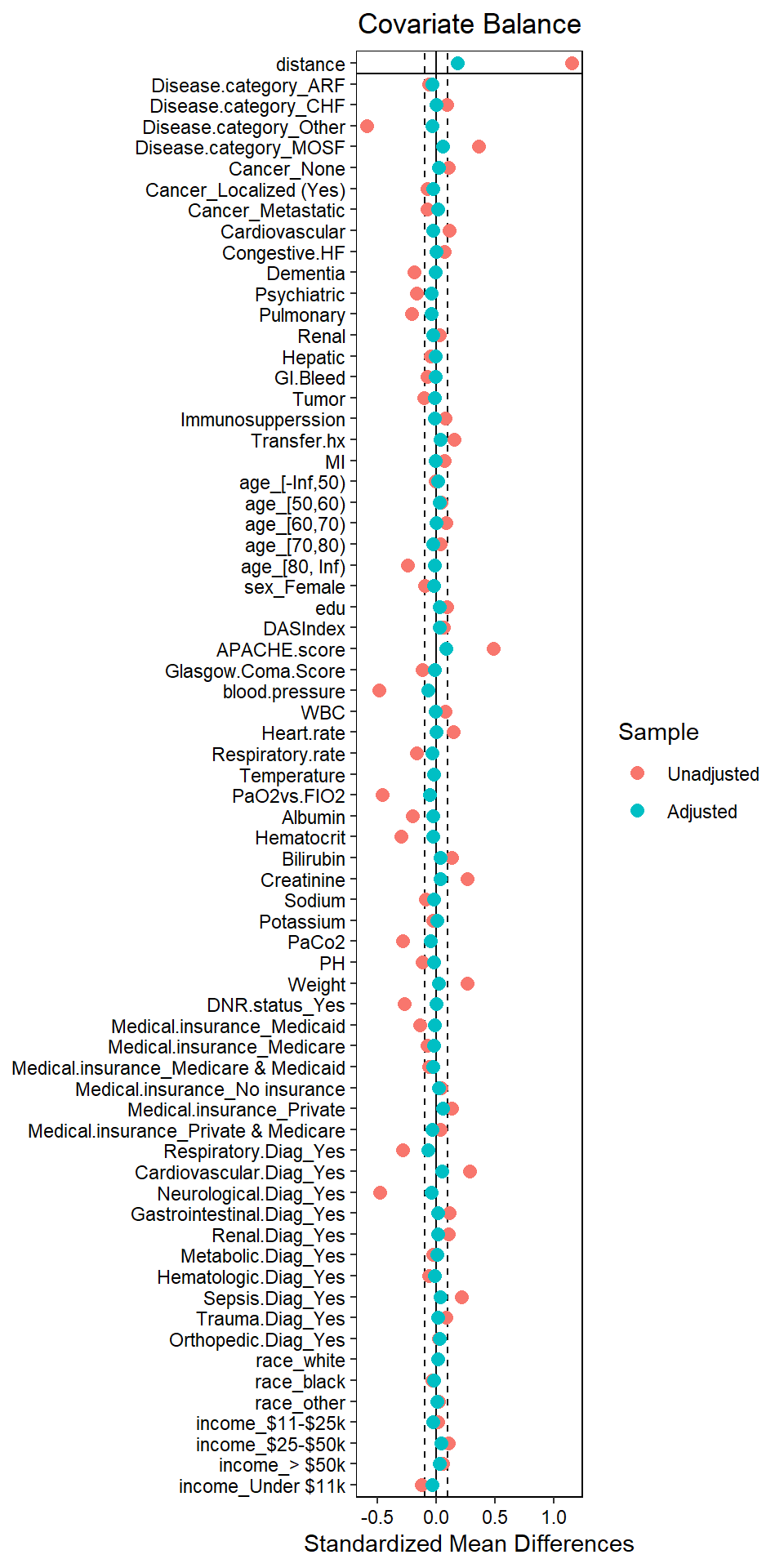
The love plot suggests satisfactory propensity score matching (all SMD < 0.1).
1.7.1.2 PSM results
1.7.1.2.1 p-value
matched.data <- match.data(match.obj)
tab1y <- CreateTableOne(vars = c("Y"),
               data = matched.data, strata = "A",
               test = TRUE)
print(tab1y, showAllLevels = FALSE,
      test = TRUE)
## Stratified by A
## 0 1 p test
## n 1739 1739
## Y (mean (SD)) 21.22 (25.36) 24.47 (28.79) <0.001Our conclusion based on propensity score pair matched data (\(p \lt 0.001\)) is different than Table 5 in Connors et al. (1996) (\(p = 0.14\)). Variability in results for 1-to-1 matching is possible, and modelling choices may be different (we used caliper option here).
1.7.1.2.2 Treatment effect
- We can also estimate the effect of
RHConlength of stayusing propensity score-matched sample:
fit.matched <- glm(Y~A,
            family=gaussian,
            data = matched.data)
publish(fit.matched)
## Variable Units Coefficient CI.95 p-value
## (Intercept) 21.22 [19.94;22.49] < 1e-04
## A 3.25 [1.45;5.05] 0.0004145saveRDS(fit.matched, file = "data/match.RDS") 1.7.2 TMLE in RHC data
There are other papers that have used RHC data (Keele and Small 2021, 2018).
Keele and Small (2021) used TMLE (with super learner SL) method in estimating the impact of RHC on length of stay, and found point estimate \(2.01 (95\% CI: 0.6-3.41)\).
In today’s workshop, we will learn about this TMLE-SL methods.
Data is freely available from Vanderbilt Biostatistics.