Chapter 4 IPTW
In this chapter, we will cover PS and IPTW (or IPW).
# Read the data saved at the last chapter
ObsData <- readRDS(file = "data/rhcAnalytic.RDS")
baselinevars <- names(dplyr::select(ObsData, !c(A,Y)))
4.1 IPTW steps
Modelling Steps:
According to Austin (2011), we need to follow 4 steps:
| Step 1 | exposure modelling: \(PS = Prob(A=1|L)\) |
| Step 2 | Convert \(PS\) to \(IPW\) = \(\frac{A}{PS} + \frac{1-A}{1-PS}\) |
| Step 3 | Assess balance in weighted sample (\(PS\) and \(L\)) |
| Step 4 | outcome modelling: \(E(Y|A=1)\) to obtain treatment effect estimate |
4.2 Step 1: exposure modelling
Exposure modelling: \(PS = Prob(A=1|L)\)
ps.formula <- as.formula(paste("A ~",
                               paste(baselinevars,
                                     collapse = "+")))
ps.formula
## A ~ Disease.category + Cancer + Cardiovascular + Congestive.HF +
## Dementia + Psychiatric + Pulmonary + Renal + Hepatic + GI.Bleed +
## Tumor + Immunosupperssion + Transfer.hx + MI + age + sex +
## edu + DASIndex + APACHE.score + Glasgow.Coma.Score + blood.pressure +
## WBC + Heart.rate + Respiratory.rate + Temperature + PaO2vs.FIO2 +
## Albumin + Hematocrit + Bilirubin + Creatinine + Sodium +
## Potassium + PaCo2 + PH + Weight + DNR.status + Medical.insurance +
## Respiratory.Diag + Cardiovascular.Diag + Neurological.Diag +
## Gastrointestinal.Diag + Renal.Diag + Metabolic.Diag + Hematologic.Diag +
## Sepsis.Diag + Trauma.Diag + Orthopedic.Diag + race + income- Other than main effect terms, what other model specifications are possible?
- Common terms to add (indeed based on biological plausibility; requiring subject area knowledge)
- Interactions
- polynomials or splines
- transformations
Fit logistic regression to estimate propensity scores
PS.fit <- glm(ps.formula,family="binomial", data=ObsData)
require(Publish)
publish(PS.fit,  format = "[u;l]")
## Variable Units OddsRatio CI.95 p-value
## Disease.category ARF Ref
## CHF 1.79 [1.32;2.43] 0.0002047
## Other 0.54 [0.43;0.68] < 1e-04
## MOSF 1.58 [1.34;1.87] < 1e-04
## Cancer None Ref
## Localized (Yes) 0.46 [0.22;0.96] 0.0389310
## Metastatic 0.37 [0.17;0.81] 0.0131229
## Cardiovascular 0 Ref
## 1 1.04 [0.86;1.25] 0.7036980
## Congestive.HF 0 Ref
## 1 1.10 [0.90;1.35] 0.3461245
## Dementia 0 Ref
## 1 0.67 [0.53;0.85] 0.0011382
## Psychiatric 0 Ref
## 1 0.65 [0.50;0.85] 0.0018616
## Pulmonary 0 Ref
## 1 0.97 [0.81;1.18] 0.7814947
## Renal 0 Ref
## 1 0.70 [0.49;1.00] 0.0523978
## Hepatic 0 Ref
## 1 0.79 [0.57;1.11] 0.1817681
## GI.Bleed 0 Ref
## 1 0.76 [0.49;1.17] 0.2148665
## Tumor 0 Ref
## 1 1.48 [0.71;3.12] 0.2987694
## Immunosupperssion 0 Ref
## 1 1.00 [0.86;1.15] 0.9778387
## Transfer.hx 0 Ref
## 1 1.46 [1.20;1.77] 0.0001356
## MI 0 Ref
## 1 1.12 [0.80;1.59] 0.5031463
## age [-Inf,50) Ref
## [50,60) 1.04 [0.85;1.27] 0.7327200
## [60,70) 1.22 [1.00;1.49] 0.0559205
## [70,80) 1.15 [0.91;1.45] 0.2414163
## [80, Inf) 0.66 [0.49;0.89] 0.0054612
## sex Male Ref
## Female 0.98 [0.86;1.12] 0.7661356
## edu 1.03 [1.01;1.05] 0.0101741
## DASIndex 1.00 [0.98;1.01] 0.6635060
## APACHE.score 1.01 [1.01;1.02] < 1e-04
## Glasgow.Coma.Score 1.00 [1.00;1.00] 0.2853053
## blood.pressure 0.99 [0.99;0.99] < 1e-04
## WBC 1.00 [0.99;1.00] 0.7368619
## Heart.rate 1.00 [1.00;1.01] < 1e-04
## Respiratory.rate 0.98 [0.97;0.98] < 1e-04
## Temperature 0.97 [0.93;1.01] 0.1255016
## PaO2vs.FIO2 0.99 [0.99;1.00] < 1e-04
## Albumin 0.93 [0.85;1.02] 0.1032557
## Hematocrit 0.99 [0.98;1.00] 0.0103236
## Bilirubin 1.01 [1.00;1.02] 0.1719966
## Creatinine 1.04 [1.00;1.09] 0.0576310
## Sodium 0.99 [0.98;1.00] 0.0049192
## Potassium 0.85 [0.79;0.91] < 1e-04
## PaCo2 0.98 [0.97;0.98] < 1e-04
## PH 0.22 [0.11;0.47] < 1e-04
## Weight 1.01 [1.00;1.01] < 1e-04
## DNR.status No Ref
## Yes 0.58 [0.46;0.73] < 1e-04
## Medical.insurance Medicaid Ref
## Medicare 1.34 [1.03;1.74] 0.0315228
## Medicare & Medicaid 1.49 [1.07;2.07] 0.0184712
## No insurance 1.66 [1.20;2.30] 0.0023684
## Private 1.55 [1.21;1.97] 0.0004402
## Private & Medicare 1.46 [1.11;1.92] 0.0071028
## Respiratory.Diag No Ref
## Yes 0.76 [0.65;0.90] 0.0010144
## Cardiovascular.Diag No Ref
## Yes 1.80 [1.52;2.13] < 1e-04
## Neurological.Diag No Ref
## Yes 0.62 [0.47;0.80] 0.0002731
## Gastrointestinal.Diag No Ref
## Yes 1.41 [1.15;1.73] 0.0010690
## Renal.Diag No Ref
## Yes 1.35 [1.01;1.80] 0.0461405
## Metabolic.Diag No Ref
## Yes 0.85 [0.63;1.15] 0.2953120
## Hematologic.Diag No Ref
## Yes 0.59 [0.45;0.78] 0.0002225
## Sepsis.Diag No Ref
## Yes 1.31 [1.10;1.57] 0.0029968
## Trauma.Diag No Ref
## Yes 3.45 [1.80;6.64] 0.0002014
## Orthopedic.Diag No Ref
## Yes 3.74 [0.53;26.25] 0.1843027
## race white Ref
## black 1.05 [0.87;1.26] 0.6250189
## other 1.09 [0.84;1.41] 0.5272282
## income $11-$25k Ref
## $25-$50k 1.08 [0.87;1.34] 0.4644703
## > $50k 1.02 [0.78;1.34] 0.8810245
## Under $11k 1.06 [0.90;1.26] 0.4797051Coef of PS model fit is not of concern.
- Model can be rich: to the extent that prediction is better
- But look for multi-collinearity issues
- SE too high?
Obtain the propesnity score (PS) values from the fit
ObsData$PS <- predict(PS.fit, type="response")
These propensity score predictions (PS) are often represented as \(g(A_i=1|L_i)\).
Check summaries:
- enough overlap?
- PS values very close to 0 or 1?
summary(ObsData$PS)## Min. 1st Qu. Median Mean 3rd Qu. Max.
## 0.002478 0.161446 0.358300 0.380819 0.574319 0.968425tapply(ObsData$PS, ObsData$A, summary)## $`0`
## Min. 1st Qu. Median Mean 3rd Qu. Max.
## 0.002478 0.106718 0.241301 0.283816 0.427138 0.951927
##
## $`1`
## Min. 1st Qu. Median Mean 3rd Qu. Max.
## 0.01575 0.37205 0.55243 0.53854 0.70999 0.96842plot(density(ObsData$PS[ObsData$A==0]),
col = "red", main = "")
lines(density(ObsData$PS[ObsData$A==1]),
col = "blue", lty = 2)
legend("topright", c("No RHC","RHC"),
col = c("red", "blue"), lty=1:2)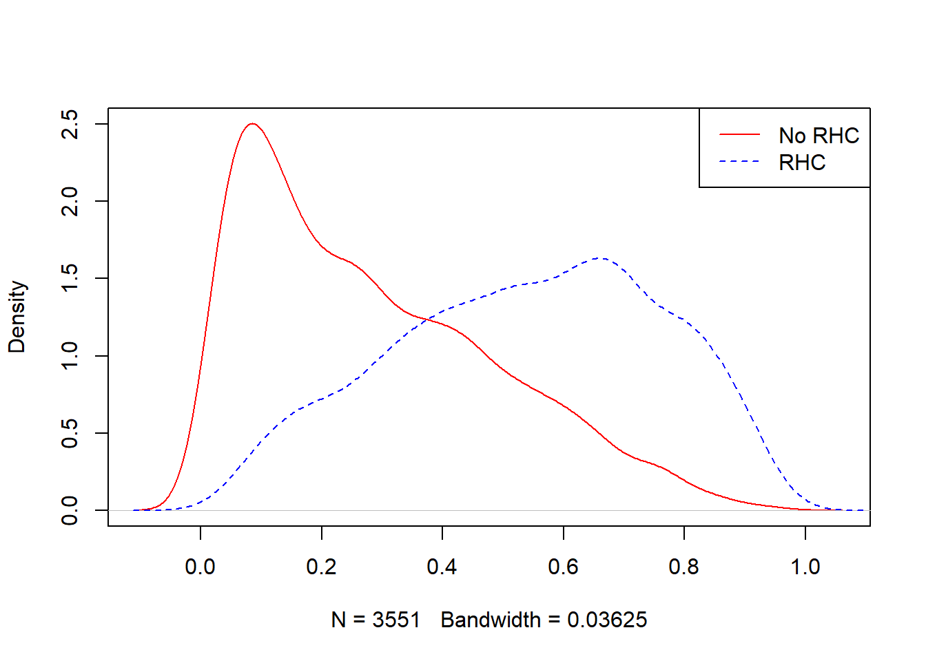
4.3 Step 2: Convert PS to IPW
Convert \(PS\) to \(IPW\) = \(\frac{A}{PS} + \frac{1-A}{1-PS}\)
- Convert PS to IPW using the formula. We are using the formula for average treatment effect (ATE).
It is possible to use alternative formulas, but we are using ATE formula for our illustration.
ObsData$IPW <- ObsData$A/ObsData$PS + (1-ObsData$A)/(1-ObsData$PS)
summary(ObsData$IPW)
## Min. 1st Qu. Median Mean 3rd Qu. Max.
## 1.002 1.183 1.472 1.986 2.064 63.509Also possible to use pre-packaged software packages to do the same:
require(WeightIt)
W.out <- weightit(ps.formula,
                    data = ObsData,
                    estimand = "ATE",
                    method = "ps")
summary(W.out$weights)
## Min. 1st Qu. Median Mean 3rd Qu. Max.
## 1.002 1.183 1.472 1.986 2.064 63.5094.4 Step 3: Balance checking
Assess balance in weighted sample (\(PS\) and \(L\))
We can check balance numerically.
- We set SMD = 0.1 as threshold for balance.
- \(SMD \gt 0.1\) means we do not have balance
require(cobalt)
bal.tab(W.out, un = TRUE,
        thresholds = c(m = .1))
## Call
## weightit(formula = ps.formula, data = ObsData, method = "ps",
## estimand = "ATE")
##
## Balance Measures
## Type Diff.Un Diff.Adj M.Threshold
## prop.score Distance 1.1926 0.0224 Balanced, <0.1
## Disease.category_ARF Binary -0.0290 0.0025 Balanced, <0.1
## Disease.category_CHF Binary 0.0261 0.0008 Balanced, <0.1
## Disease.category_Other Binary -0.1737 -0.0080 Balanced, <0.1
## Disease.category_MOSF Binary 0.1766 0.0047 Balanced, <0.1
## Cancer_None Binary 0.0439 0.0017 Balanced, <0.1
## Cancer_Localized (Yes) Binary -0.0267 0.0017 Balanced, <0.1
## Cancer_Metastatic Binary -0.0172 -0.0034 Balanced, <0.1
## Cardiovascular Binary 0.0445 0.0051 Balanced, <0.1
## Congestive.HF Binary 0.0268 0.0013 Balanced, <0.1
## Dementia Binary -0.0472 -0.0138 Balanced, <0.1
## Psychiatric Binary -0.0348 -0.0050 Balanced, <0.1
## Pulmonary Binary -0.0737 -0.0058 Balanced, <0.1
## Renal Binary 0.0066 0.0027 Balanced, <0.1
## Hepatic Binary -0.0124 -0.0012 Balanced, <0.1
## GI.Bleed Binary -0.0122 -0.0026 Balanced, <0.1
## Tumor Binary -0.0423 -0.0016 Balanced, <0.1
## Immunosupperssion Binary 0.0358 -0.0027 Balanced, <0.1
## Transfer.hx Binary 0.0554 0.0047 Balanced, <0.1
## MI Binary 0.0139 0.0005 Balanced, <0.1
## age_[-Inf,50) Binary -0.0017 -0.0098 Balanced, <0.1
## age_[50,60) Binary 0.0161 0.0149 Balanced, <0.1
## age_[60,70) Binary 0.0355 -0.0108 Balanced, <0.1
## age_[70,80) Binary 0.0144 0.0047 Balanced, <0.1
## age_[80, Inf) Binary -0.0643 0.0010 Balanced, <0.1
## sex_Female Binary -0.0462 -0.0143 Balanced, <0.1
## edu Contin. 0.0914 -0.0000 Balanced, <0.1
## DASIndex Contin. 0.0626 0.0435 Balanced, <0.1
## APACHE.score Contin. 0.5014 0.0109 Balanced, <0.1
## Glasgow.Coma.Score Contin. -0.1098 0.0034 Balanced, <0.1
## blood.pressure Contin. -0.4551 0.0057 Balanced, <0.1
## WBC Contin. 0.0836 0.0470 Balanced, <0.1
## Heart.rate Contin. 0.1469 0.0210 Balanced, <0.1
## Respiratory.rate Contin. -0.1655 0.0037 Balanced, <0.1
## Temperature Contin. -0.0214 0.0090 Balanced, <0.1
## PaO2vs.FIO2 Contin. -0.4332 -0.0016 Balanced, <0.1
## Albumin Contin. -0.2299 -0.0279 Balanced, <0.1
## Hematocrit Contin. -0.2693 -0.0247 Balanced, <0.1
## Bilirubin Contin. 0.1446 -0.0069 Balanced, <0.1
## Creatinine Contin. 0.2696 0.0148 Balanced, <0.1
## Sodium Contin. -0.0922 -0.0059 Balanced, <0.1
## Potassium Contin. -0.0271 -0.0264 Balanced, <0.1
## PaCo2 Contin. -0.2486 -0.0201 Balanced, <0.1
## PH Contin. -0.1198 0.0095 Balanced, <0.1
## Weight Contin. 0.2557 0.0209 Balanced, <0.1
## DNR.status_Yes Binary -0.0696 -0.0112 Balanced, <0.1
## Medical.insurance_Medicaid Binary -0.0395 0.0058 Balanced, <0.1
## Medical.insurance_Medicare Binary -0.0327 -0.0119 Balanced, <0.1
## Medical.insurance_Medicare & Medicaid Binary -0.0144 -0.0001 Balanced, <0.1
## Medical.insurance_No insurance Binary 0.0099 -0.0002 Balanced, <0.1
## Medical.insurance_Private Binary 0.0624 0.0013 Balanced, <0.1
## Medical.insurance_Private & Medicare Binary 0.0143 0.0052 Balanced, <0.1
## Respiratory.Diag_Yes Binary -0.1277 -0.0056 Balanced, <0.1
## Cardiovascular.Diag_Yes Binary 0.1395 0.0034 Balanced, <0.1
## Neurological.Diag_Yes Binary -0.1079 -0.0038 Balanced, <0.1
## Gastrointestinal.Diag_Yes Binary 0.0453 -0.0028 Balanced, <0.1
## Renal.Diag_Yes Binary 0.0264 0.0021 Balanced, <0.1
## Metabolic.Diag_Yes Binary -0.0059 0.0002 Balanced, <0.1
## Hematologic.Diag_Yes Binary -0.0146 -0.0000 Balanced, <0.1
## Sepsis.Diag_Yes Binary 0.0912 0.0035 Balanced, <0.1
## Trauma.Diag_Yes Binary 0.0105 0.0011 Balanced, <0.1
## Orthopedic.Diag_Yes Binary 0.0010 0.0002 Balanced, <0.1
## race_white Binary 0.0063 -0.0030 Balanced, <0.1
## race_black Binary -0.0114 0.0067 Balanced, <0.1
## race_other Binary 0.0050 -0.0036 Balanced, <0.1
## income_$11-$25k Binary 0.0062 -0.0096 Balanced, <0.1
## income_$25-$50k Binary 0.0391 0.0032 Balanced, <0.1
## income_> $50k Binary 0.0165 -0.0001 Balanced, <0.1
## income_Under $11k Binary -0.0618 0.0065 Balanced, <0.1
##
## Balance tally for mean differences
## count
## Balanced, <0.1 69
## Not Balanced, >0.1 0
##
## Variable with the greatest mean difference
## Variable Diff.Adj M.Threshold
## WBC 0.047 Balanced, <0.1
##
## Effective sample sizes
## Control Treated
## Unadjusted 3551. 2184.
## Adjusted 2532.46 1039.44- We can also check this in a plot
require(cobalt)
love.plot(W.out, binary = "std",
          thresholds = c(m = .1),
          abs = TRUE,
          var.order = "unadjusted",
          line = TRUE)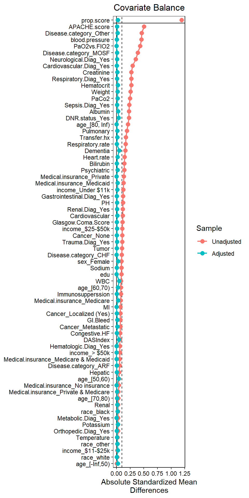
All covariates are balanced! Reverse engineered an RCT!?!
4.5 Step 4: outcome modelling
Outcome modelling: \(E(Y|A=1)\) to obtain treatment effect estimate
Estimate the effect of treatment on outcomes
out.formula <- as.formula(Y ~ A)
out.fit <- glm(out.formula,
               data = ObsData,
               weights = IPW)
publish(out.fit)
## Variable Units Coefficient CI.95 p-value
## (Intercept) 20.68 [19.73;21.64] < 1e-04
## A 3.24 [1.88;4.60] < 1e-04saveRDS(out.fit, file = "data/ipw.RDS")
We are now primarily interested about exposure modelling (e.g., fixing imbalance first, before doing outcome analysis).