Chapter 8 Final Words

8.1 Select variables judiciously

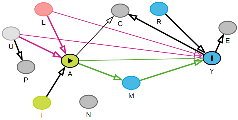
Figure 8.1: Variable roles: A = exposure or treatment; Y = outcome; L = confounder; R = risk factor for Y; M = mediator; C = collider; E = effect of Y; I = instrument; u = unmeasured confounder; P = proxy of U; N = noise variable

• Think about the role of variables first
  • ideally include confounders to reduce bias
  • consider including risk factor for outcome for greater accuracy
  • IV, collider, mediators, effect of outcome, noise variables should be avoided
  • if something is unmeasured, consider adding proxy (with caution)
• If you do not have subject area expertise, talk to experts
• do pre-screening
  • sparse binary variables
  • highly collinear variables

Relying on just a blackbox ML method may be dangerous to identify the roles of variables in the relationship of interest.

8.2 Why SL and TMLE

8.2.1 Prediction goal

• Assuming all covariates are measured, parametric models such as linear and logistic regressions are very efficient, but relies on strong assumptions. In real-world scenarios, it is often hard (if not impossible) to guess the correct specification of the right hand side of the regression equation.
• Machine learning (ML) methods are very helpful for prediction goals. They are also helpful in identifying complex functions (non-linearities and non-additive terms) of the covariates (again, assuming they are measured).
• There are many ML methods, but the procedures are very different, and they come with their own advantages and disadvantages. In a given real data, it is hard to apriori predict which is the best ML algorithm for a given problem.

Super learner is helpful in combining strength from various algorithms, and producing 1 prediction column that has optimal statistical properties.

8.2.2 Causal inference

• For causal inference goals (when we have a primary exposure of interest), machine learning methods are often misleading. This is primarily due to the fact that they usually do not have an inherent mechanism of focusing on primary exposure (RHC in this example); and treats the primary exposure as any other predictors.
• When using g-computation with ML methods, estimation of variance becomes a difficult problem (with correct coverage). Generalized procedures such as robust SE or bootstrap methods are not supported by theory.

TMLE method shine, with the help of it’s important statistical properties (double robustness, finite sample properties).

8.2.3 Identifiability assumptions

However, causal inference requires satisfying identifiability assumptions for us to interpret causality based on association measures from statistical models (see below). Many of these assumptions are not empirically testable. That is why, it is extremely important to work with subject area experts to assess the plausibility of those assumptions in the given context.

No ML method, no matter how fancy it is, can automatically produce estimates that can be directly interpreted as causal, unless the identifiability assumptions are properly taken into account.

Conditional Exchangeability	\(Y(1), Y(0) \perp A | L\)	Treatment assignment is independent of the potential outcome, given covariates
Positivity	\(0 < P(A=1 | L) < 1\)	Subjects are eligible to receive both treatment, given covariates
Consistency	\(Y = Y(a) \forall A=a\)	No multiple version of the treatment; and well defined treatment

8.3 Further reading

8.3.1 Key articles

• TMLE Procedure:
  • Luque-Fernandez et al. (2018)
  • Schuler and Rose (2017)
• Super learner:
  • Rose (2013)
  • Naimi and Balzer (2018)

8.3.2 Additional readings

• Rose (2020)
• Snowden, Rose, and Mortimer (2011)
• Naimi, Cole, and Kennedy (2017)
• Austin and Stuart (2015)
• Naimi, Mishler, and Kennedy (2017)
• Balzer and Westling (2021)

8.3.3 Workshops

Highly recommend joining SER if interested in Epi methods development. The following workshops and summer course are very useful.

• SER Workshop Targeted Learning: Causal Inference Meets Machine Learning by Alan Hubbard Mark van der Laan, 2021
• SER Workshop Introduction to Parametric and Semi-parametric Estimators for Causal Inference by Laura B. Balzer & Jennifer Ahern, 2020
• SER Workshop Machine Learning and Artificial Intelligence for Causal Inference and Prediction: A Primer by Naimi A, 2021
• SISCER Modern Statistical Learning for Observational Data by Marco Carone, David Benkeser, 2021

8.3.4 Recorded webinars

The following webinars and workshops are freely accessible, and great for understanding the intuitions, theories and mechanisms behind these methods!

8.3.4.1 Introductory materials

• An Introduction to Targeted Maximum Likelihood Estimation of Causal Effects by Susan Gruber (Putnam Data Sciences)
• Practical Considerations for Specifying a Super Learner by Rachael Phillips (Putnam Data Sciences)

8.3.4.2 More theory talks

• Targeted Machine Learning for Causal Inference based on Real World Data by Mark van der Laan (Putnam Data Sciences)
• An introduction to Super Learning by Eric Polly (Putnam Data Sciences)
• Cross-validated Targeted Maximum Likelihood Estimation (CV-TMLE) by Alan Hubbard (Putnam Data Sciences)
• Higher order Targeted Maximum Likelihood Estimation by Mark van der Laan (Online Causal Inference Seminar)
• Targeted learning for the estimation of drug safety and effectiveness: Getting better answers by asking better questions by Mireille Schnitzer (CNODES)

8.3.4.3 More applied talks

• Applications of Targeted Maximum Likelihood Estimation by Laura Balzar (UCSF Epi & Biostats)
• Applying targeted maximum likelihood estimation to pharmacoepidemiology by Menglan Pang (CNODES)

8.3.4.4 Blog

• Kat’s Stats by Katherine Hoffman
• towardsdatascience by Yao Yang
• The Research Group of Mark van der Laan by Mark van der Laan

References

Austin, Peter C, and Elizabeth A Stuart. 2015. “Moving Towards Best Practice When Using Inverse Probability of Treatment Weighting (IPTW) Using the Propensity Score to Estimate Causal Treatment Effects in Observational Studies.” Statistics in Medicine 34 (28): 3661–79.

Balzer, Laura B, and Ted Westling. 2021. “Demystifying Statistical Inference When Using Machine Learning in Causal Research.” American Journal of Epidemiology.

Luque-Fernandez, Miguel Angel, Michael Schomaker, Bernard Rachet, and Mireille E Schnitzer. 2018. “Targeted Maximum Likelihood Estimation for a Binary Treatment: A Tutorial.” Statistics in Medicine 37 (16): 2530–46.

Naimi, Ashley I, and Laura B Balzer. 2018. “Stacked Generalization: An Introduction to Super Learning.” European Journal of Epidemiology 33 (5): 459–64.

Naimi, Ashley I, Stephen R Cole, and Edward H Kennedy. 2017. “An Introduction to g Methods.” International Journal of Epidemiology 46 (2): 756–62.

Naimi, Ashley I, Alan E Mishler, and Edward H Kennedy. 2017. “Challenges in Obtaining Valid Causal Effect Estimates with Machine Learning Algorithms.” arXiv Preprint arXiv:1711.07137.

Rose, Sherri. 2013. “Mortality Risk Score Prediction in an Elderly Population Using Machine Learning.” American Journal of Epidemiology 177 (5): 443–52.

———. 2020. “Intersections of Machine Learning and Epidemiological Methods for Health Services Research.” International Journal of Epidemiology 49 (6): 1763–70.

Schuler, Megan S, and Sherri Rose. 2017. “Targeted Maximum Likelihood Estimation for Causal Inference in Observational Studies.” American Journal of Epidemiology 185 (1): 65–73.

Snowden, Jonathan M, Sherri Rose, and Kathleen M Mortimer. 2011. “Implementation of g-Computation on a Simulated Data Set: Demonstration of a Causal Inference Technique.” American Journal of Epidemiology 173 (7): 731–38.