Chapter 5 IPTW using ML
Similar to G-computation, we will try to use machine learning methods, particularly Superlearner in estimating IPW estimates
# Read the data saved at the last chapter
ObsData <- readRDS(file = "data/rhcAnalytic.RDS")
baselinevars <- names(dplyr::select(ObsData, !c(A,Y)))
ps.formula <- as.formula(paste("A ~",
                               paste(baselinevars,
                                     collapse = "+")))
5.1 IPTW Steps from SL
Modelling Steps:
We will still follow the same steps
| Step 1 | exposure modelling: \(PS = Prob(A=1|L)\) |
| Step 2 | Convert \(PS\) to \(IPW\) = \(\frac{A}{PS} + \frac{1-A}{1-PS}\) |
| Step 3 | Assess balance in weighted sample and overlap (\(PS\) and \(L\)) |
| Step 4 | outcome modelling: \(Prob(Y=1|A=1)\) to obtain treatment effect estimate |
5.2 Step 1: exposure modelling
This is the exposure model that we decided on:
ps.formula## A ~ Disease.category + Cancer + Cardiovascular + Congestive.HF +
## Dementia + Psychiatric + Pulmonary + Renal + Hepatic + GI.Bleed +
## Tumor + Immunosupperssion + Transfer.hx + MI + age + sex +
## edu + DASIndex + APACHE.score + Glasgow.Coma.Score + blood.pressure +
## WBC + Heart.rate + Respiratory.rate + Temperature + PaO2vs.FIO2 +
## Albumin + Hematocrit + Bilirubin + Creatinine + Sodium +
## Potassium + PaCo2 + PH + Weight + DNR.status + Medical.insurance +
## Respiratory.Diag + Cardiovascular.Diag + Neurological.Diag +
## Gastrointestinal.Diag + Renal.Diag + Metabolic.Diag + Hematologic.Diag +
## Sepsis.Diag + Trauma.Diag + Orthopedic.Diag + race + incomeWe again use the same candidate learners:
- linear model
- LASSO
- gradient boosting
require(SuperLearner)
ObsData.noYA <- dplyr::select(ObsData, !c(Y,A))
PS.fit.SL <- SuperLearner(Y=ObsData$A,
                       X=ObsData.noYA,
                       cvControl = list(V = 3),
                       SL.library=c("SL.glm", "SL.glmnet", "SL.xgboost"),
                       method="method.NNLS",
                       family="binomial")
Here, method.AUC is also possible to use instead of method.NNLS for binary response. We could use cvControl = list(V = 3, stratifyCV = TRUE) to make the splits be stratified by the binary response.
Obtain the propesnity score (PS) values from the fit
all.pred <- predict(PS.fit.SL, type = "response")
ObsData$PS.SL <- all.pred$pred
Check summaries:
summary(ObsData$PS.SL)## V1
## Min. :0.002981
## 1st Qu.:0.151578
## Median :0.347286
## Mean :0.380833
## 3rd Qu.:0.591373
## Max. :0.971231tapply(ObsData$PS.SL, ObsData$A, summary)## $`0`
## Min. 1st Qu. Median Mean 3rd Qu. Max.
## 0.002981 0.091153 0.192876 0.224573 0.332211 0.788300
##
## $`1`
## Min. 1st Qu. Median Mean 3rd Qu. Max.
## 0.0815 0.5107 0.6510 0.6349 0.7663 0.9712plot(density(ObsData$PS.SL[ObsData$A==0]),
col = "red", main = "")
lines(density(ObsData$PS.SL[ObsData$A==1]),
col = "blue", lty = 2)
legend("topright", c("No RHC","RHC"),
col = c("red", "blue"), lty=1:2)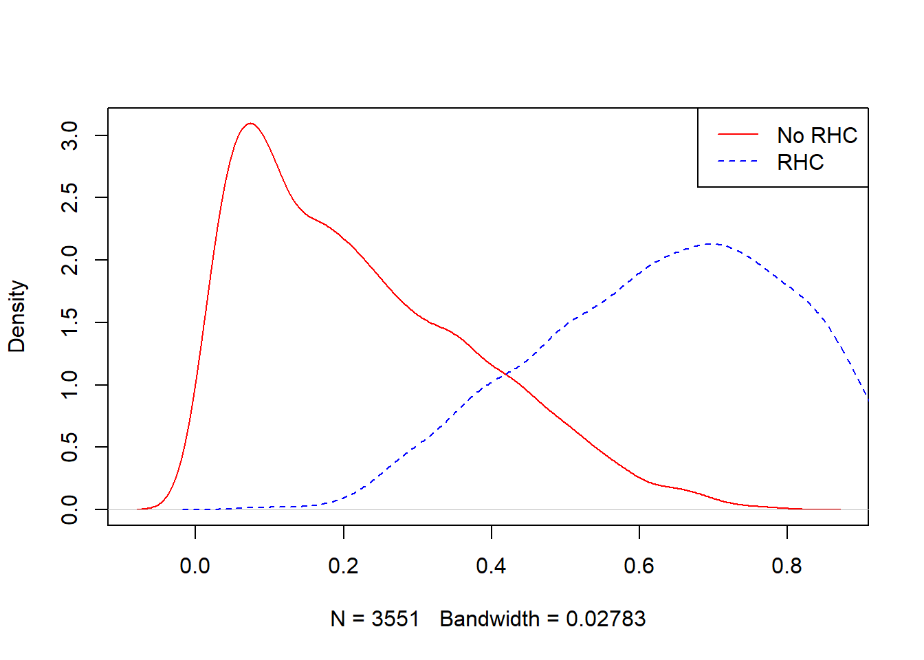
5.3 Step 2: Convert PS to IPW
- Convert PS from SL to IPW using the formula (again, ATE formula).
ObsData$IPW.SL <- ObsData$A/ObsData$PS.SL + (1-ObsData$A)/(1-ObsData$PS.SL)
summary(ObsData$IPW.SL)
## V1
## Min. : 1.003
## 1st Qu.: 1.149
## Median : 1.339
## Mean : 1.508
## 3rd Qu.: 1.668
## Max. :12.271Output from pre-packged software packages to do the same (very similar estimates):
require(WeightIt)
W.out <- weightit(ps.formula,
                    data = ObsData,
                    estimand = "ATE",
                    method = "super",
                    SL.library = c("SL.glm",
                                   "SL.glmnet",
                                   "SL.xgboost"))
summary(W.out$weights)
## Min. 1st Qu. Median Mean 3rd Qu. Max.
## 1.002 1.141 1.321 1.471 1.626 12.435saveRDS(W.out, file = "data/ipwslps.RDS")Alternatively, you can use the previously estimated PS
W.out2 <- weightit(ps.formula,
                    data = ObsData,
                    estimand = "ATE",
                    ps = ObsData$PS.SL)
summary(W.out2$weights)
## Min. 1st Qu. Median Mean 3rd Qu. Max.
## 1.003 1.149 1.339 1.508 1.668 12.2715.4 Step 3: Balance checking
- We first check balance numerically for SMD = 0.1 as threshold for balance.
bal.tab(W.out, un = TRUE,
        thresholds = c(m = .1))
## Call
## weightit(formula = ps.formula, data = ObsData, method = "super",
## estimand = "ATE", SL.library = c("SL.glm", "SL.glmnet", "SL.xgboost"))
##
## Balance Measures
## Type Diff.Un Diff.Adj
## prop.score Distance 2.7115 2.1229
## Disease.category_ARF Binary -0.0290 -0.0094
## Disease.category_CHF Binary 0.0261 0.0153
## Disease.category_Other Binary -0.1737 -0.1013
## Disease.category_MOSF Binary 0.1766 0.0954
## Cancer_None Binary 0.0439 0.0249
## Cancer_Localized (Yes) Binary -0.0267 -0.0120
## Cancer_Metastatic Binary -0.0172 -0.0129
## Cardiovascular Binary 0.0445 0.0283
## Congestive.HF Binary 0.0268 0.0161
## Dementia Binary -0.0472 -0.0296
## Psychiatric Binary -0.0348 -0.0204
## Pulmonary Binary -0.0737 -0.0430
## Renal Binary 0.0066 0.0046
## Hepatic Binary -0.0124 -0.0082
## GI.Bleed Binary -0.0122 -0.0081
## Tumor Binary -0.0423 -0.0230
## Immunosupperssion Binary 0.0358 0.0200
## Transfer.hx Binary 0.0554 0.0281
## MI Binary 0.0139 0.0075
## age_[-Inf,50) Binary -0.0017 -0.0014
## age_[50,60) Binary 0.0161 0.0130
## age_[60,70) Binary 0.0355 0.0167
## age_[70,80) Binary 0.0144 0.0112
## age_[80, Inf) Binary -0.0643 -0.0396
## sex_Female Binary -0.0462 -0.0283
## edu Contin. 0.0914 0.0512
## DASIndex Contin. 0.0626 0.0378
## APACHE.score Contin. 0.5014 0.2641
## Glasgow.Coma.Score Contin. -0.1098 -0.0603
## blood.pressure Contin. -0.4551 -0.2406
## WBC Contin. 0.0836 0.0503
## Heart.rate Contin. 0.1469 0.0819
## Respiratory.rate Contin. -0.1655 -0.0829
## Temperature Contin. -0.0214 -0.0060
## PaO2vs.FIO2 Contin. -0.4332 -0.2339
## Albumin Contin. -0.2299 -0.1292
## Hematocrit Contin. -0.2693 -0.1590
## Bilirubin Contin. 0.1446 0.0771
## Creatinine Contin. 0.2696 0.1425
## Sodium Contin. -0.0922 -0.0513
## Potassium Contin. -0.0271 -0.0284
## PaCo2 Contin. -0.2486 -0.1483
## PH Contin. -0.1198 -0.0533
## Weight Contin. 0.2557 0.1418
## DNR.status_Yes Binary -0.0696 -0.0426
## Medical.insurance_Medicaid Binary -0.0395 -0.0224
## Medical.insurance_Medicare Binary -0.0327 -0.0184
## Medical.insurance_Medicare & Medicaid Binary -0.0144 -0.0065
## Medical.insurance_No insurance Binary 0.0099 0.0062
## Medical.insurance_Private Binary 0.0624 0.0333
## Medical.insurance_Private & Medicare Binary 0.0143 0.0077
## Respiratory.Diag_Yes Binary -0.1277 -0.0673
## Cardiovascular.Diag_Yes Binary 0.1395 0.0760
## Neurological.Diag_Yes Binary -0.1079 -0.0592
## Gastrointestinal.Diag_Yes Binary 0.0453 0.0249
## Renal.Diag_Yes Binary 0.0264 0.0148
## Metabolic.Diag_Yes Binary -0.0059 -0.0027
## Hematologic.Diag_Yes Binary -0.0146 -0.0084
## Sepsis.Diag_Yes Binary 0.0912 0.0485
## Trauma.Diag_Yes Binary 0.0105 0.0064
## Orthopedic.Diag_Yes Binary 0.0010 0.0007
## race_white Binary 0.0063 0.0034
## race_black Binary -0.0114 -0.0043
## race_other Binary 0.0050 0.0009
## income_$11-$25k Binary 0.0062 0.0007
## income_$25-$50k Binary 0.0391 0.0211
## income_> $50k Binary 0.0165 0.0078
## income_Under $11k Binary -0.0618 -0.0296
## M.Threshold
## prop.score
## Disease.category_ARF Balanced, <0.1
## Disease.category_CHF Balanced, <0.1
## Disease.category_Other Not Balanced, >0.1
## Disease.category_MOSF Balanced, <0.1
## Cancer_None Balanced, <0.1
## Cancer_Localized (Yes) Balanced, <0.1
## Cancer_Metastatic Balanced, <0.1
## Cardiovascular Balanced, <0.1
## Congestive.HF Balanced, <0.1
## Dementia Balanced, <0.1
## Psychiatric Balanced, <0.1
## Pulmonary Balanced, <0.1
## Renal Balanced, <0.1
## Hepatic Balanced, <0.1
## GI.Bleed Balanced, <0.1
## Tumor Balanced, <0.1
## Immunosupperssion Balanced, <0.1
## Transfer.hx Balanced, <0.1
## MI Balanced, <0.1
## age_[-Inf,50) Balanced, <0.1
## age_[50,60) Balanced, <0.1
## age_[60,70) Balanced, <0.1
## age_[70,80) Balanced, <0.1
## age_[80, Inf) Balanced, <0.1
## sex_Female Balanced, <0.1
## edu Balanced, <0.1
## DASIndex Balanced, <0.1
## APACHE.score Not Balanced, >0.1
## Glasgow.Coma.Score Balanced, <0.1
## blood.pressure Not Balanced, >0.1
## WBC Balanced, <0.1
## Heart.rate Balanced, <0.1
## Respiratory.rate Balanced, <0.1
## Temperature Balanced, <0.1
## PaO2vs.FIO2 Not Balanced, >0.1
## Albumin Not Balanced, >0.1
## Hematocrit Not Balanced, >0.1
## Bilirubin Balanced, <0.1
## Creatinine Not Balanced, >0.1
## Sodium Balanced, <0.1
## Potassium Balanced, <0.1
## PaCo2 Not Balanced, >0.1
## PH Balanced, <0.1
## Weight Not Balanced, >0.1
## DNR.status_Yes Balanced, <0.1
## Medical.insurance_Medicaid Balanced, <0.1
## Medical.insurance_Medicare Balanced, <0.1
## Medical.insurance_Medicare & Medicaid Balanced, <0.1
## Medical.insurance_No insurance Balanced, <0.1
## Medical.insurance_Private Balanced, <0.1
## Medical.insurance_Private & Medicare Balanced, <0.1
## Respiratory.Diag_Yes Balanced, <0.1
## Cardiovascular.Diag_Yes Balanced, <0.1
## Neurological.Diag_Yes Balanced, <0.1
## Gastrointestinal.Diag_Yes Balanced, <0.1
## Renal.Diag_Yes Balanced, <0.1
## Metabolic.Diag_Yes Balanced, <0.1
## Hematologic.Diag_Yes Balanced, <0.1
## Sepsis.Diag_Yes Balanced, <0.1
## Trauma.Diag_Yes Balanced, <0.1
## Orthopedic.Diag_Yes Balanced, <0.1
## race_white Balanced, <0.1
## race_black Balanced, <0.1
## race_other Balanced, <0.1
## income_$11-$25k Balanced, <0.1
## income_$25-$50k Balanced, <0.1
## income_> $50k Balanced, <0.1
## income_Under $11k Balanced, <0.1
##
## Balance tally for mean differences
## count
## Balanced, <0.1 59
## Not Balanced, >0.1 9
##
## Variable with the greatest mean difference
## Variable Diff.Adj M.Threshold
## APACHE.score 0.2641 Not Balanced, >0.1
##
## Effective sample sizes
## Control Treated
## Unadjusted 3551. 2184.
## Adjusted 3316.37 1896.5- And also via plot
require(cobalt)
love.plot(W.out, binary = "std",
          thresholds = c(m = .1),
          abs = TRUE,
          var.order = "unadjusted",
          line = TRUE)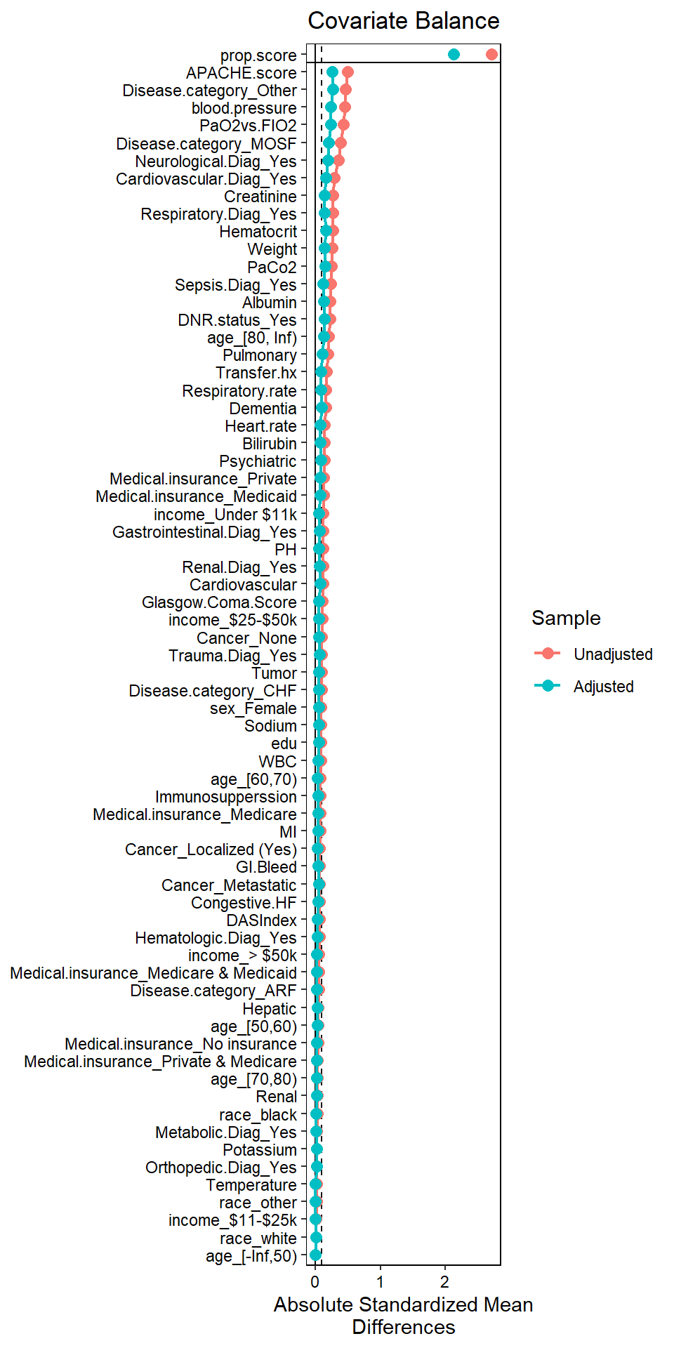
Some covariates have SMD > 0.1 (sign of imbalance). This phenomenon is common when we use strong ML methods to obtain PS (Alam, Moodie, and Stephens 2019).
5.5 Step 4: outcome modelling
Estimate the effect of treatment on outcomes
5.5.1 Crude
out.formula <- as.formula(Y ~ A)
out.fit <- glm(out.formula,
               data = ObsData,
               weights = IPW.SL)
publish(out.fit)
## Variable Units Coefficient CI.95 p-value
## (Intercept) 20.21 [19.31;21.12] < 1e-04
## A 4.24 [2.88;5.61] < 1e-045.5.2 Adjusted
Adjusting for all covariates to deal with potential residual confounding (as was indicated by imbalance). Alternatively, could adjust for selected covariates believed to be the reasons for potential imbalance (Nguyen et al. 2017).
Estimate the effect of treatment on outcomes (after adjustment)
out.formula2 <- as.formula(paste("Y~ A +",
                               paste(baselinevars,
                                     collapse = "+")))
out.fit2 <- glm(out.formula2,
               data = ObsData,
               weights = IPW.SL)
res2 <- publish(out.fit2, digits=1)$regressionTable[2,]res2| Variable | Units | Coefficient | CI.95 | p-value |
|---|---|---|---|---|
| A | 2.9 | [1.5;4.3] | <0.1 |
5.5.3 Adjusted (from package)
Also check the output when we used the weights from the package
out.fit3 <- glm(out.formula2,
               data = ObsData,
               weights = W.out$weights)
res3 <- publish(out.fit3, digits=1)$regressionTable[2,]res3| Variable | Units | Coefficient | CI.95 | p-value |
|---|---|---|---|---|
| A | 2.9 | [1.5;4.3] | <0.1 |
saveRDS(out.fit3, file = "data/ipwsl.RDS")
Fit SuperLearner (SL) to estimate propensity scores.