Chapter 7 Unsupervised Learning
- Watch the video describing this chapter
Clustering is an unsupervised learning algorithm. These algorithms can classify data into multiple groups. Such classification is based on similarity.
Group characteristics include (to the extent that is possible)
- low inter-class similarity: observation from different clusters would be dissimilar
- high intra-class similarity: observation from the same cluster would be similar
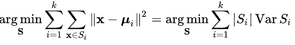
Within-cluster variation will be thus minimized by optimizing within-cluster sum of squares of Euclidean distances (ref)
7.1 K-means
K-means is a very popular clustering algorithm, that partitions the data into \(k\) groups.
Algorithm:
- Determine a number \(k\) (e.g., could be 3)
- randomly select \(k\) subjects in a data. Use these points as staring points (centers or cluster mean) for each cluster.
- By Euclidean distance measure (from the initial centers), try to determine in which cluster the remaining points belong.
- compute new mean value for each cluster.
- based on this new mean, try to determine again in which cluster the data points belong.
- process continues until the data points do not change cluster membership.
7.2 Read previously saved data
ObsData <- readRDS(file = "data/rhcAnalytic.RDS")7.2.1 Example 1
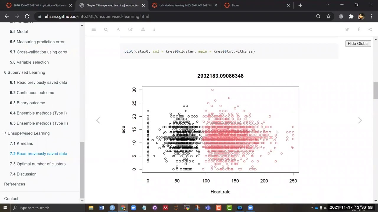
datax0 <- ObsData[c("Heart.rate", "edu")]
kres0 <- kmeans(datax0, centers = 2, nstart = 10)
kres0$centers
## Heart.rate edu
## 1 54.55138 11.44494
## 2 134.96277 11.75466plot(datax0, col = kres0$cluster, main = kres0$tot.withinss)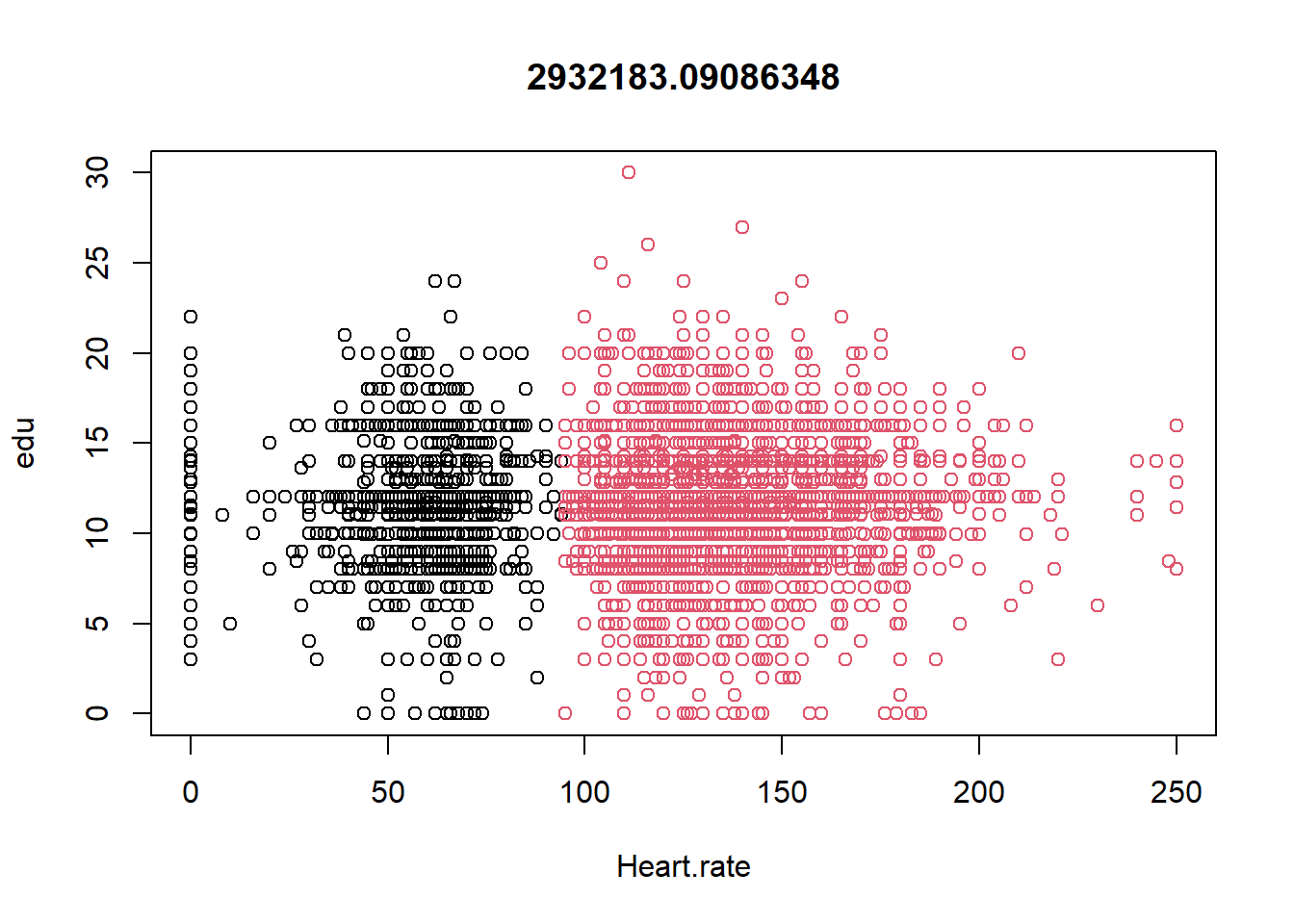
7.2.2 Example 2
datax0 <- ObsData[c("blood.pressure", "Heart.rate",
                    "Respiratory.rate")]
kres0 <- kmeans(datax0, centers = 2, nstart = 10)
kres0$centers
## blood.pressure Heart.rate Respiratory.rate
## 1 80.10812 135.08956 29.85267
## 2 73.71684 54.95789 22.76723plot(datax0, col = kres0$cluster, main = kres0$tot.withinss)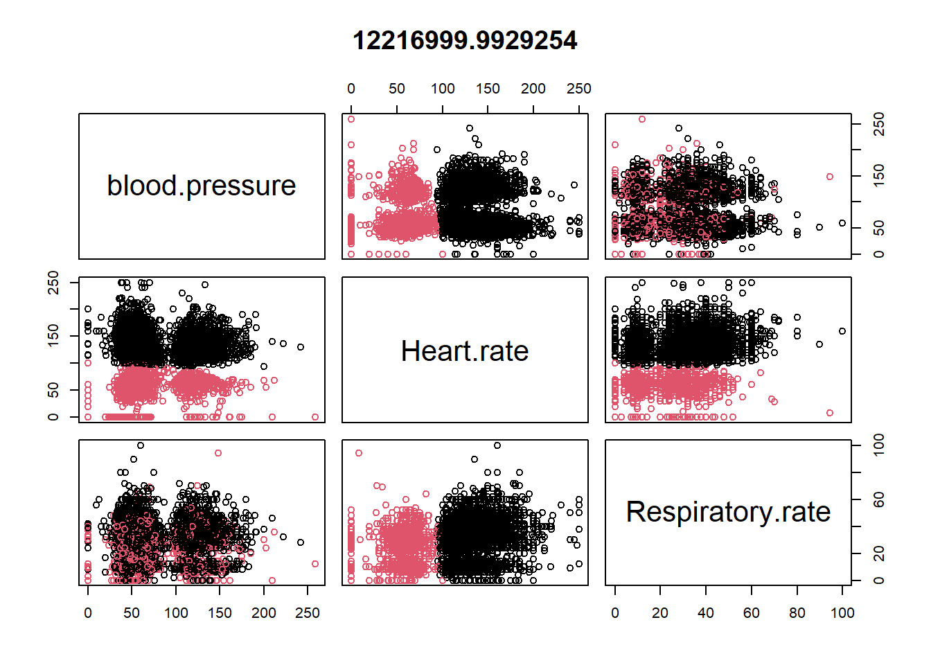
7.2.3 Example with many variables
datax <- ObsData[c("edu", "blood.pressure", "Heart.rate",
                   "Respiratory.rate" , "Temperature",
                   "PH", "Weight", "Length.of.Stay")]
kres <- kmeans(datax, centers = 3)
#kres
head(kres$cluster)## [1] 1 1 1 3 1 2kres$size## [1] 2793 1688 1254kres$centers## edu blood.pressure Heart.rate Respiratory.rate Temperature PH
## 1 11.85833 54.26924 136.37451 29.76119 37.85078 7.385249
## 2 11.54214 128.33886 126.12026 29.36611 37.68129 7.401027
## 3 11.46134 65.47249 53.24242 22.65973 37.01597 7.378482
## Weight Length.of.Stay
## 1 68.63384 23.42356
## 2 66.68351 20.68128
## 3 67.57291 18.58931aggregate(datax, by = list(cluster = kres$cluster), mean)## cluster edu blood.pressure Heart.rate Respiratory.rate Temperature
## 1 1 11.85833 54.26924 136.37451 29.76119 37.85078
## 2 2 11.54214 128.33886 126.12026 29.36611 37.68129
## 3 3 11.46134 65.47249 53.24242 22.65973 37.01597
## PH Weight Length.of.Stay
## 1 7.385249 68.63384 23.42356
## 2 7.401027 66.68351 20.68128
## 3 7.378482 67.57291 18.58931aggregate(datax, by = list(cluster = kres$cluster), sd)## cluster edu blood.pressure Heart.rate Respiratory.rate Temperature
## 1 1 3.162485 11.93763 23.13140 13.67791 1.781692
## 2 2 3.091605 18.58070 27.68369 14.08169 1.610746
## 3 3 3.160538 31.89150 23.63993 13.60831 1.832389
## PH Weight Length.of.Stay
## 1 0.1082140 27.99506 29.01143
## 2 0.1009567 32.15078 23.37223
## 3 0.1226041 26.87075 20.820247.3 Optimal number of clusters
require(factoextra)
fviz_nbclust(datax, kmeans, method = "wss")+
  geom_vline(xintercept=3,linetype=3)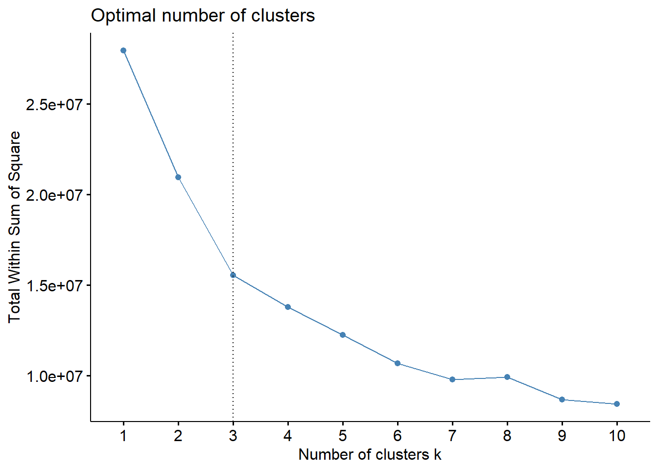
Here the vertical line is chosen based on elbow method (ref).
7.4 Discussion
- We need to supply a number, \(k\): but we can test different \(k\)s to identify optimal value
- Clustering can be influenced by outliners, so median based clustering is possible
-
mere ordering can influence clustering, hence we should choose
different initial means (e.g.,
nstartshould be greater than 1).
In this chapter, we will talk about unsupervised learning.