Chapter 3 Data spliting
- Watch the video describing this chapter
3.1 Read previously saved data
ObsData <- readRDS(file = "data/rhcAnalytic.RDS")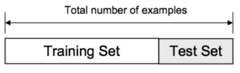
# Using a seed to randomize in a reproducible way
set.seed(123)
require(caret)
split<-createDataPartition(y = ObsData$Length.of.Stay,
                           p = 0.7, list = FALSE)
str(split)
## int [1:4017, 1] 1 2 3 4 5 6 7 8 9 10 ...
## - attr(*, "dimnames")=List of 2
## ..$ : NULL
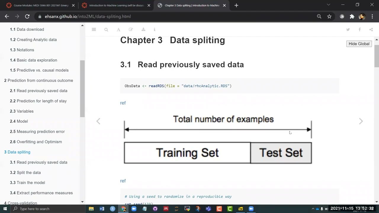
## ..$ : chr "Resample1"dim(split)## [1] 4017 1dim(ObsData)*.7 # approximate train data## [1] 4014.5 36.4dim(ObsData)*(1-.7) # approximate train data## [1] 1720.5 15.63.2 Split the data
# create train data
train.data<-ObsData[split,]
dim(train.data)
## [1] 4017 52# create test data
test.data<-ObsData[-split,]
dim(test.data)## [1] 1718 523.3 Train the model
out.formula1 <- readRDS(file = "data/form1.RDS")
out.formula1
## Length.of.Stay ~ Disease.category + Cancer + Cardiovascular +
## Congestive.HF + Dementia + Psychiatric + Pulmonary + Renal +
## Hepatic + GI.Bleed + Tumor + Immunosupperssion + Transfer.hx +
## MI + age + sex + edu + DASIndex + APACHE.score + Glasgow.Coma.Score +
## blood.pressure + WBC + Heart.rate + Respiratory.rate + Temperature +
## PaO2vs.FIO2 + Albumin + Hematocrit + Bilirubin + Creatinine +
## Sodium + Potassium + PaCo2 + PH + Weight + DNR.status + Medical.insurance +
## Respiratory.Diag + Cardiovascular.Diag + Neurological.Diag +
## Gastrointestinal.Diag + Renal.Diag + Metabolic.Diag + Hematologic.Diag +
## Sepsis.Diag + Trauma.Diag + Orthopedic.Diag + race + income +
## RHC.usefit.train1<-lm(out.formula1, data = train.data)
# summary(fit.train1)3.3.1 Function that gives performance measures
perform <- function(new.data,
                    model.fit,model.formula=NULL,
                    y.name = "Y",
                    digits=3){
  # data dimension
  p <- dim(model.matrix(model.fit))[2]
  # predicted value
  pred.y <- predict(model.fit, new.data)
  # sample size
  n <- length(pred.y)
  # outcome
  new.data.y <- as.numeric(new.data[,y.name])
  # R2
  R2 <- caret:::R2(pred.y, new.data.y)
  # adj R2 using alternate formula
  df.residual <- n-p
  adjR2 <- 1-(1-R2)*((n-1)/df.residual)
  # RMSE
  RMSE <-  caret:::RMSE(pred.y, new.data.y)
  # combine all of the results
  res <- round(cbind(n,p,R2,adjR2,RMSE),digits)
  # returning object
  return(res)
}
3.4 Extract performance measures
perform(new.data=train.data,
        y.name = "Length.of.Stay",
        model.fit=fit.train1)
## n p R2 adjR2 RMSE
## [1,] 4017 64 0.081 0.067 24.647perform(new.data=test.data,
y.name = "Length.of.Stay",
model.fit=fit.train1)## n p R2 adjR2 RMSE
## [1,] 1718 64 0.056 0.02 25.488perform(new.data=ObsData,
y.name = "Length.of.Stay",
model.fit=fit.train1)## n p R2 adjR2 RMSE
## [1,] 5735 64 0.073 0.063 24.902
In this chapter, we will describe the ideas of internal validation.