require(twangContinuous)
set.seed(1235)
data(dat)
summary(dat$tss_0) # treatment
#>    Min. 1st Qu.  Median    Mean 3rd Qu.    Max.
#> 0.000 0.000 0.000 2.101 4.000 13.0005 Continuous exposure
Steps
- We use the same 4 steps for the propensity score weighting analysis when the exposure is continuous.
- exposure modelling needs to be handled by generalized linear models that can accommodate continuous scale exposure.
5.1 Step 1: Estimation of Propensity scores via GBM
test.mod <- ps.cont(tss_0 ~ sfs8p_0 + sati_0 + sp_sm_0
                    + recov_0 + subsgrps_n + treat,
                    data=dat,
                    n.trees = 500,
                    shrinkage = 0.01,
                    interaction.depth = 3,
                    verbose = FALSE)
twangContinuous::bal.table(test.mod, digits = 3)
5.2 Step 2: IPW calculation for ATT
dat$wts <- twangContinuous::get.weights(test.mod)
summary(dat$wts)
#>    Min. 1st Qu.  Median    Mean 3rd Qu.    Max.
#> 0.04231 0.85715 0.90552 0.99339 1.05425 6.31356
# by(dat$wts, dat$tss_0, summary)
5.3 Step 3: Balance assessment in weighted data
Tip
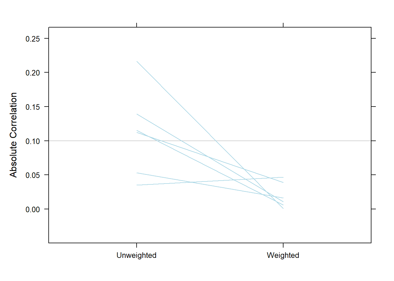
Based on absolute Pearson correlation between the exposure and each confounder
bal.table(test.mod, digits = 3)plot(test.mod, plots="es")
5.4 Step 4: Effect estimates from weighted outcome model
design.ps <- svydesign(ids=~1, weights=~wts, data=dat)
outcome.model <- svyglm(sfs8p_3 ~ tss_0, design = design.ps,
                        family = gaussian())
publish(outcome.model, intercept = FALSE, digits = 4)
#>  Variable Units Coefficient            CI.95  p-value
#>     tss_0            0.0026 [-0.1197;0.1249]   0.9666