4 Categorical exposure
Steps
- We use the same 4 steps for the propensity score weighting analysis when the exposure is multi-category.
- exposure modelling needs to be handled by generalized linear models that can accommodate multi-categories of exposure.
4.1 Alcohol and Other Drug treatment data
require(twang)
data(AOD)
head(AOD)table(AOD$treat)
#>
#> community metcbt5 scy
#> 200 200 200Here,
- Outcome variable: suf12: substance use frequency at 12 month follow-up
- exposure variable: treat: possible values
- community: traditional programs (community)
- metcbt5: evidence-based MET/CBT-5 treatment protocol
- scy: Strengthening Communities for Youth
- Covariates (pre-treatment):
- illact: illicit activities scale
- crimjust: criminal justice involvement
- subprob: substance use problem scale
- subdep: substance use dependence scale
- white: non-Hispanic white youth
4.2 Step 1: Estimation of Propensity scores
We can fit vector generalized linear models (VGLMs) to fit propensity score model with our 3 category exposure variable:
require(VGAM)
psFormula <- "treat ~ illact + crimjust + subprob + subdep + white"
ps.model <- vglm(psFormula,family=multinomial, data=AOD)
AOD$ps <- data.frame(fitted(ps.model))require(ggplot2)
ggplot(AOD, aes(x=ps[,1], fill=factor(treat))) +
geom_density(alpha=0.5) +
scale_fill_discrete(name="Treatment Group") +
labs(title="Density Plot of Propensity Scores by Treatment Group",
x="Propensity Score",
y="Density") +
theme_minimal()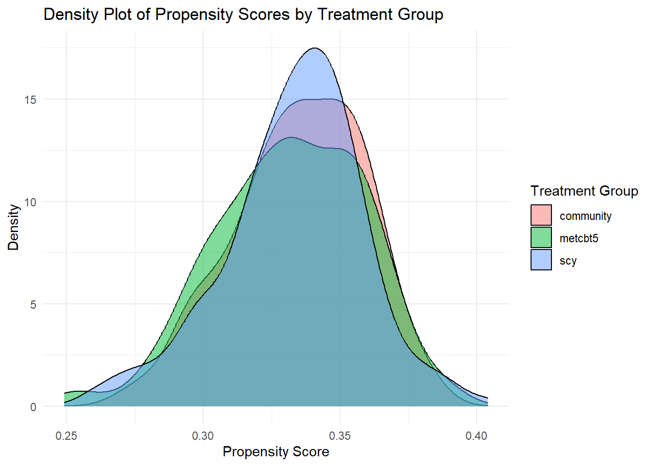
4.3 Step 1: Estimation of Propensity scores via GBM
set.seed(1235)
mnps.AOD.ATT <- mnps(treat ~ illact + crimjust + subprob + subdep + white,
                 data = AOD,
                 interaction.depth = 3,
                 estimand = "ATT",
                 treatATT = "community", # the treated
                 verbose = FALSE,
                 stop.method = "es.mean",
                 n.trees = 1000)
4.4 Step 2: IPW calculation for ATT
AOD$w.ATT <- twang::get.weights(mnps.AOD.ATT, stop.method = "es.mean")
summary(AOD$w.ATT)
#>    Min. 1st Qu.  Median    Mean 3rd Qu.    Max.
#>  0.1494  0.7265  1.0000  0.8896  1.0000  1.8823
by(AOD$w.ATT, AOD$treat, summary)
#> AOD$treat: community
#>    Min. 1st Qu.  Median    Mean 3rd Qu.    Max.
#>       1       1       1       1       1       1
#> ------------------------------------------------------------
#> AOD$treat: metcbt5
#>    Min. 1st Qu.  Median    Mean 3rd Qu.    Max.
#>  0.1494  0.4939  0.7204  0.7529  0.9460  1.8386
#> ------------------------------------------------------------
#> AOD$treat: scy
#>    Min. 1st Qu.  Median    Mean 3rd Qu.    Max.
#>  0.3548  0.7619  0.9630  0.9159  1.0263  1.8823
4.5 Step 3: Balance assessment in weighted data
Tip
Stopping rules specified earlier has 2 components:
- a balance metric (for covariates) and
- rule for summarizing (across covariates).
twang::bal.table(mnps.AOD.ATT,
                 digits = 2,
                 collapse.to = "covariate")[,c("max.std.eff.sz",
"stop.method")]plot(mnps.AOD.ATT, plots = 3)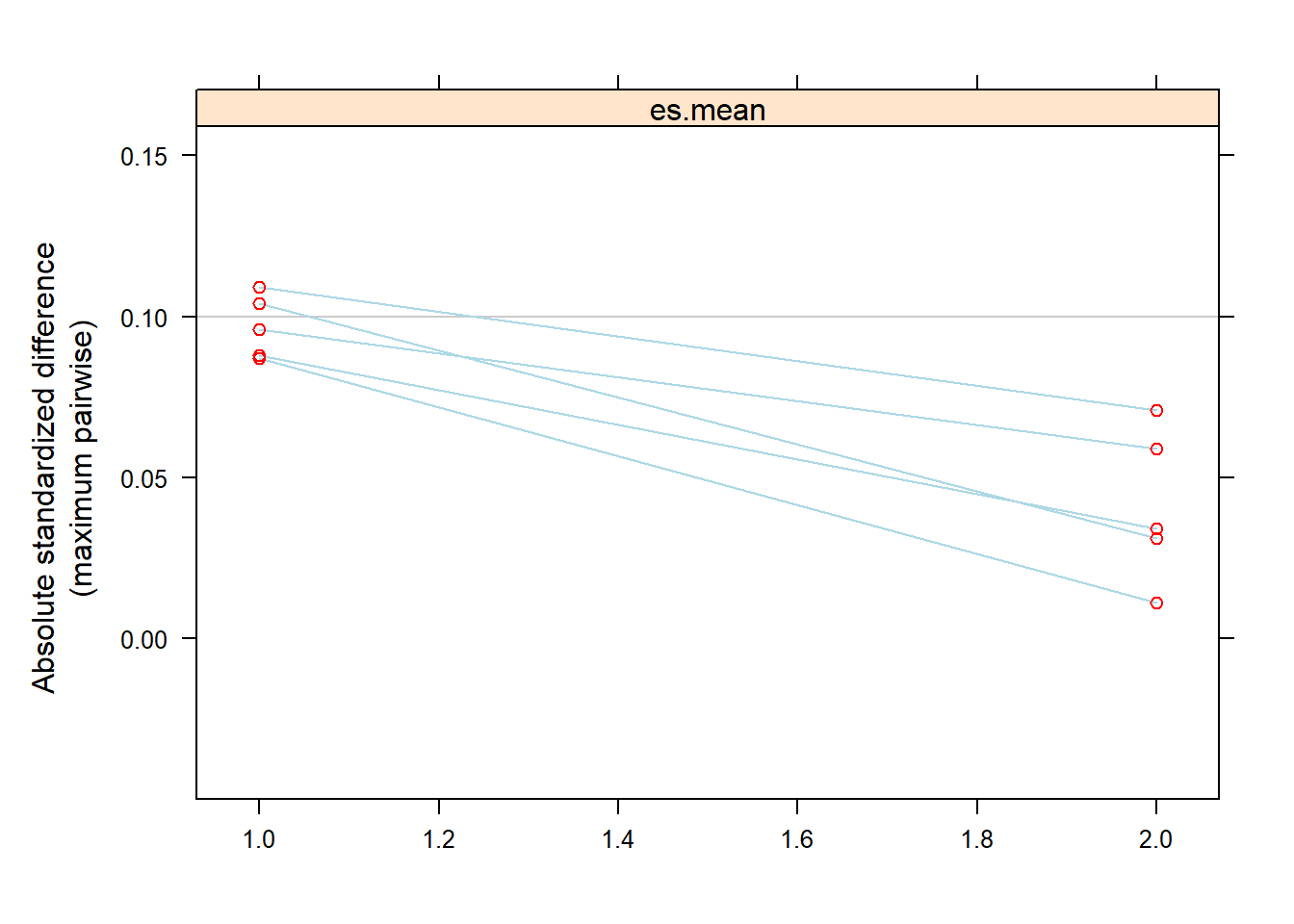
4.6 Step 4: Effect estimates from weighted outcome model
require(survey)
design.mnps.ATT <- svydesign(ids=~1, weights=~w.ATT, data=AOD)
fit <- svyglm(suf12 ~ treat, design = design.mnps.ATT)
require(Publish)
publish(fit, intercept = FALSE)
#>  Variable     Units Coefficient        CI.95   p-value
#>     treat community         Ref
#>             metcbt5        0.20 [-0.00;0.41]   0.05129
#>                 scy        0.08 [-0.11;0.27]   0.41503