Survival Analysis with svyTable1

knitr::opts_chunk$set(
  collapse = TRUE,
  comment = "#>"
)

This vignette introduces survival analysis tools in the svyTable1 package for complex survey data. The functions support Kaplan–Meier estimation, proportional hazards diagnostics, and multiple imputation pipelines.

The vignette covers three tasks:

Visualizing survival curves with svykmplot()
Testing the proportional hazards assumption with an ad-hoc procedure svycoxph_CE()
Extending proportional hazards diagnostics to multiply imputed data with svycoxph_CE_mi()

1. Visualizing Survey-Weighted Survival Data (`svykmplot`)

library(svyTable1)
library(survey)
library(knitr)
library(survival)
library(ggplot2)
library(dplyr)
library(mitools)
library(mice)

svykmplot() produces Kaplan–Meier survival estimates that correctly incorporate survey weights, strata, and clusters. The function returns both a plot and a number-at-risk table. The plot supports automatic or custom colors, p-value display, and censoring indicators.

The example below uses the NHANES linked mortality file to compare survival across levels of caffeine consumption among women.

The number-at-risk table is printed beneath the plot, which is required by common reporting guidelines.

data(nhanes_mortality)

analytic_design <- svydesign(
  strata = ~strata,
  id = ~psu,
  weights = ~survey_weight,
  data = nhanes_mortality,
  nest = TRUE
)

design_female <- subset(analytic_design, sex == "Female")

km_formula <- Surv(stime, status) ~ caff

distinct_palette <- c("#377EB8", "#FF7F00", "#4DAF4A", "#E41A1C")

km_results_female <- svykmplot(
  formula = km_formula,
  design = design_female,
  legend_title = "Caffeine Consumption",
  time_unit = "days",
  time_breaks = seq(0, 240, by = 60),
  palette = distinct_palette,
  show_pval = TRUE,
  show_censor_marks = TRUE
)

km_results_female$plot
#> Warning: Removed 1 row containing missing values or values outside the scale range
#> (`geom_step()`).
#> Warning: Removed 1 row containing missing values or values outside the scale range
#> (`geom_ribbon()`).
#> Warning: Removed 38 rows containing missing values or values outside the scale range
#> (`geom_point()`).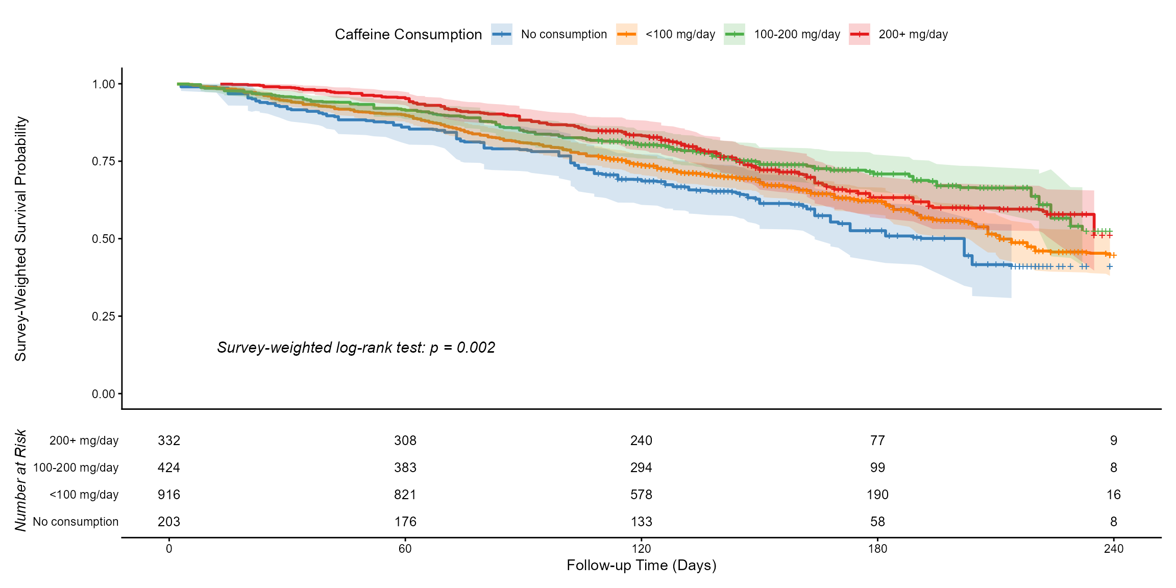

knitr::kable(
  km_results_female$table,
  caption = "Number at Risk for Female Mortality Plot"
)

2. Ad hoc solutions for testing Proportional Hazards

The R functions, svycoxph_CE (for single survey designs) and svycoxph_CE_mi (for multiply imputed survey designs), are ad hoc solutions for testing the Proportional Hazards (PH) assumption in a complex survey data analysis environment.

What the Functions Do

Both functions implement the same core strategy for assessing the PH assumption, which is violated if the effect of a covariate changes over time (i.e., $\beta(t) \neq \beta$ ). They transform the proportional hazards model (second equation below) into a time-dependent coefficient model using a step-function approach.

The fundamental Cox models are:

Proportional Hazards (PH):
$\lambda(t) = \lambda_{0}(t) e^{\beta X}$
Time-Dependent Coefficient:
$\lambda(t) = \lambda_{0}(t) e^{\beta(t)X}$

The step-function approach works by:

Defining Time Intervals:
The total follow-up time is split into $n$ distinct intervals (for example, 5 quantiles of event times).
Splitting the Data:
The input dataset is expanded into a start-stop format using survival::survSplit(). A single subject’s follow-up is broken into multiple rows, one for each time interval they contribute to.
Fitting Interval-Specific Models:
A separate Cox model is fitted for each time interval. This is achieved by including a term such as
var_to_test:strata(tgroup)
or by subsetting the data by the interval variable (tgroup) and using
Surv(tstart, time, status) ~ ... in the model formula.
Multiple Imputation Support:
For svycoxph_CE_mi, each interval model is pooled across the multiple imputations using mitools::pool().
Extracting and Plotting Coefficients:
The functions extract the coefficient ( $\hat{\beta}$ ) and its standard error for the variable being tested across intervals, then plot them against time.

Interpretation

If the true effect is constant (PH holds), the plotted coefficients should cluster around the overall constant-effect estimate, with confidence intervals overlapping the overall mean or null-effect line.
A clear time trend in the step-function coefficients suggests a PH violation.

Why These are Ad Hoc Solutions, and Why the Specialized Functions are Necessary

The svycoxph_CE and svycoxph_CE.mi functions are “ad hoc” solutions; and they are purpose-built to solve a gap in R’s survival analysis ecosystem. Standard methods for testing the proportional hazards assumption fail when faced with the combined complexity of survey design, multiple imputation, and time-varying coefficients.

This function is the correct solution because it successfully navigates three distinct incompatibilities in standard packages:

Incompatibility of cox.zph() and svycoxph

The standard function cox.zph() (based on Schoenfeld residuals) cannot be used on svycoxph objects. Using it on a non-survey coxph model, even with a weights() term, ignores the clusters and strata, leading to incorrect standard errors and invalid p-values.

Potential Solution: The svycoxph_CE functions use svycoxph for every calculation, ensuring that the survey design’s variance estimation is correctly applied at all steps.

Incompatibility of tt() and svycoxph

The “correct” way to model a continuously time-varying coefficient (e.g., $\beta(t) = a + b \log(t)$ ) in a coxph model is to use the tt() (time-transform) argument.

The Problem: The tt() argument is not implemented in the survey::svycoxph function. A researcher using survey data is therefore technically blocked from using this method.
Potential Solution: The step-function approach is the most robust, non-parametric alternative. By fitting separate models in discrete time intervals, it makes no assumptions about the shape of the effect over time and is fully compatible with svycoxph.

Incompatibility of cox.zph() and Multiple Imputation

Standard diagnostics like cox.zph() are not designed to be “pooled” across multiply-imputed datasets. A researcher might incorrectly run the test on just one imputed dataset or, worse, on the stacked (long-format) data, both of which are invalid.

Potential Solution: The svycoxph_CE.mi function correctly handles multiple imputation by fitting the step-function model separately to each imputed dataset and then pooling the results using Rubin’s Rules (mitools::pool()). This produces a single, valid estimate and confidence interval for the coefficient in each time interval.

Avoiding the “Obvious but Incorrect” log(t) Trap

It is a common mistake (Therneau, Crowson, and Atkinson 2017) to test the PH assumption by adding a simple interaction like covariate:log(time) to the formula.

The Problem: This is statistically invalid, as it introduces circular logic. It uses the subject’s final follow-up time (part of the outcome) as a predictor for the hazard at all earlier time points .
Potential Solution: The survSplit method avoids this by partitioning the data into (start, stop] intervals. The model at any given interval t only uses data from subjects still at risk, correctly adhering to the principles of survival analysis.

Complete case (`svycoxph_CE`)

data(nhanes_mortality)

analytic_design <- svydesign(
  strata = ~strata,
  id = ~psu,
  weights = ~survey_weight,
  data = nhanes_mortality,
  nest = TRUE
)

data_full_clean <- analytic_design$variables %>%
  dplyr::filter(stime > 0) %>%
  mutate(
    caff_bin = factor(
      ifelse(caff == "No consumption", "No", "Yes"),
      levels = c("No", "Yes")
    )
  )

analytic_design_final <- svydesign(
  strata = ~strata,
  id = ~psu,
  weights = ~survey_weight,
  data = data_full_clean,
  nest = TRUE
)

my_formula <- "caff_bin + age"
my_var <- "age"

svycoxph_CE(
  formula_rhs = my_formula,
  design = analytic_design_final,
  var_to_test = my_var,
  time_var = "stime",
  status_var = "status",
  n_intervals = 5,
  verbose = TRUE,
  print_main_model = TRUE,
  print_split_summary = TRUE
)
#> [1] "--- Fitting Main (Constant Effect) Model ---"
#> Stratified 1 - level Cluster Sampling design (with replacement)
#> With (180) clusters.
#> svydesign(strata = ~strata, id = ~psu, weights = ~survey_weight, 
#>     data = data_full_clean, nest = TRUE)
#> 
#> 
#> |Variable    |    HR| CI.Lower| CI.Upper| p.value|
#> |:-----------|-----:|--------:|--------:|-------:|
#> |caff_binYes | 0.764|    0.622|    0.938|    0.01|
#> |age         | 1.075|    1.067|    1.082|    0.00|
#> 
#> [1] "--- Cut points used ---"
#> 20% 40% 60% 80% 
#>  42  75 106 144 
#> [1] "--- Using Automatic Design Extraction ---"
#> Stratified 1 - level Cluster Sampling design (with replacement)
#> With (180) clusters.
#> subset(split_design, split_design$variables$tgroup == i)
#> Stratified 1 - level Cluster Sampling design (with replacement)
#> With (180) clusters.
#> subset(split_design, split_design$variables$tgroup == i)
#> Stratified 1 - level Cluster Sampling design (with replacement)
#> With (180) clusters.
#> subset(split_design, split_design$variables$tgroup == i)
#> Stratified 1 - level Cluster Sampling design (with replacement)
#> With (180) clusters.
#> subset(split_design, split_design$variables$tgroup == i)
#> Stratified 1 - level Cluster Sampling design (with replacement)
#> With (139) clusters.
#> subset(split_design, split_design$variables$tgroup == i)
#> [1] "--- Summary of Time-Interval Models ---"
#> 
#> 
#> |Time.Interval |Variable    |    HR| CI.Lower| CI.Upper| p.value|
#> |:-------------|:-----------|-----:|--------:|--------:|-------:|
#> |0-42          |caff_binYes | 0.625|    0.433|    0.903|   0.012|
#> |0-42          |age         | 1.077|    1.062|    1.093|   0.000|
#> |42-75         |caff_binYes | 0.768|    0.459|    1.284|   0.314|
#> |42-75         |age         | 1.064|    1.051|    1.078|   0.000|
#> |75-106        |caff_binYes | 0.911|    0.569|    1.461|   0.700|
#> |75-106        |age         | 1.074|    1.059|    1.089|   0.000|
#> |106-144       |caff_binYes | 0.832|    0.507|    1.365|   0.467|
#> |106-144       |age         | 1.085|    1.070|    1.101|   0.000|
#> |144-249       |caff_binYes | 0.735|    0.462|    1.170|   0.195|
#> |144-249       |age         | 1.075|    1.059|    1.090|   0.000|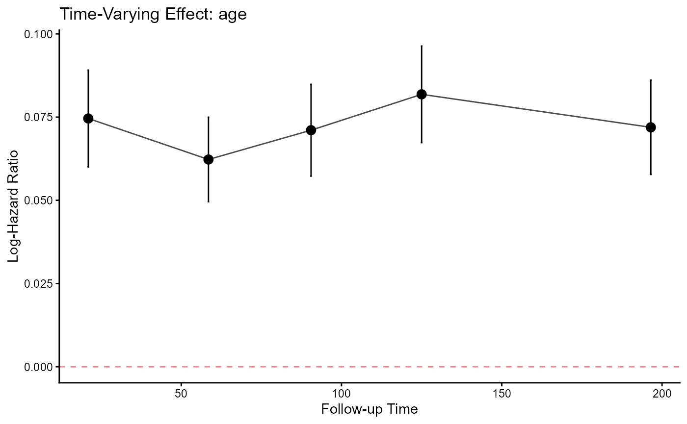

Multiple Imputation Case (svycoxph_CE_mi)

data(nhanes_mortality)

analytic_design <- svydesign(
  strata = ~strata,
  id = ~psu,
  weights = ~survey_weight,
  data = nhanes_mortality,
  nest = TRUE
)

set.seed(123)
data_with_miss <- analytic_design$variables %>%
  dplyr::filter(stime > 0) %>%
  mutate(
    caff_bin = factor(
      ifelse(caff == "No consumption", "No", "Yes"),
      levels = c("No", "Yes")
    ),
    age = ifelse(runif(n()) < 0.10, NA, age),
    bmi_cat = factor(ifelse(age > 50 & runif(n()) < 0.15, NA, as.character(bmi.cat)))
  )

print(mice::md.pattern(data_with_miss[, c("age", "bmi_cat", "caff_bin", "stime", "status")], plot = FALSE))
#>      caff_bin stime status age bmi_cat    
#> 2994        1     1      1   1       1   0
#> 401         1     1      1   1       0   1
#> 343         1     1      1   0       1   1
#> 42          1     1      1   0       0   2
#>             0     0      0 385     443 828

data_with_miss$nelson_aalen <- nelsonaalen(
  data_with_miss,
  time = stime,
  status = status
)

M_IMPUTATIONS <- 2
MAX_ITERATIONS <- 2

pred_matrix <- make.predictorMatrix(data_with_miss)
vars_to_keep_as_is <- c("id", "survey.weight", "psu", "strata",
                        "stime", "status", "nelson_aalen", "caff_bin", "sex")

pred_matrix[, vars_to_keep_as_is] <- 0
pred_matrix[vars_to_keep_as_is, ] <- 0

imputed_data <- mice(
  data_with_miss,
  m = M_IMPUTATIONS,
  maxit = MAX_ITERATIONS,
  predictorMatrix = pred_matrix,
  method = "pmm",
  seed = 123,
  printFlag = FALSE
)
#> Warning: Number of logged events: 4

impdata_long <- mice::complete(imputed_data, "long", include = FALSE)

allImputations_main <- imputationList(split(impdata_long, impdata_long$.imp))
design_main <- svydesign(
  strata = ~strata,
  id = ~psu,
  weights = ~survey_weight,
  data = allImputations_main,
  nest = TRUE
)

my_formula <- "caff_bin + sex + age + bmi_cat"
main_formula <- as.formula(paste0("Surv(stime, status) ~ ", my_formula))

main_fit_list <- with(design_main, svycoxph(main_formula))
main_fit_pooled <- pool(main_fit_list)
#> Stratified 1 - level Cluster Sampling design (with replacement)
#> With (180) clusters.
#> svydesign(ids = ids, probs = probs, strata = strata, variables = variables, 
#>     fpc = fpc, nest = nest, check.strata = check.strata, weights = weights, 
#>     data = d, pps = pps, calibrate.formula = calibrate.formula, 
#>     ...)
#> Stratified 1 - level Cluster Sampling design (with replacement)
#> With (180) clusters.
#> svydesign(ids = ids, probs = probs, strata = strata, variables = variables, 
#>     fpc = fpc, nest = nest, check.strata = check.strata, weights = weights, 
#>     data = d, pps = pps, calibrate.formula = calibrate.formula, 
#>     ...)
#> Stratified 1 - level Cluster Sampling design (with replacement)
#> With (180) clusters.
#> svydesign(ids = ids, probs = probs, strata = strata, variables = variables, 
#>     fpc = fpc, nest = nest, check.strata = check.strata, weights = weights, 
#>     data = d, pps = pps, calibrate.formula = calibrate.formula, 
#>     ...)

event_times <- data_with_miss$stime[data_with_miss$status == 1]
cuts <- quantile(event_times, probs = c(0.2, 0.4, 0.6, 0.8), na.rm = TRUE)

impdata_long_split <- survSplit(Surv(stime, status) ~ .,
                                data = impdata_long,
                                cut = cuts,
                                episode = "tgroup",
                                id = "split_id")

allImputations_split <- imputationList(split(impdata_long_split, impdata_long_split$.imp))

design_split <- svydesign(
  strata = ~strata,
  id = ~psu,
  weights = ~survey_weight,
  data = allImputations_split,
  nest = TRUE
)

my_ph_plot <- svycoxph_CE_mi(
  formula_rhs = my_formula,
  design_split = design_split,
  var_to_test = "caff_binYes",
  tgroup_var = "tgroup",
  time_var = "stime",
  status_var = "status",
  main_model_fit = main_fit_pooled,
  print_split_summary = TRUE,
  show_null_effect = TRUE
)
#> [1] "--- Tidy Table for Final Paper (if Constant Effect Assumption is Met) ---"
#> 
#> 
#> |Variable             |    HR| CI.Lower| CI.Upper| p.value|
#> |:--------------------|-----:|--------:|--------:|-------:|
#> |caff_binYes          | 0.797|   -0.445|   -0.010|   0.041|
#> |sexFemale            | 0.701|   -0.511|   -0.199|   0.000|
#> |age                  | 1.071|    0.061|    0.076|   0.000|
#> |bmi_cat20.0 to <25.0 | 0.342|   -1.613|   -0.534|   0.000|
#> |bmi_cat25.0 to <30.0 | 0.287|   -1.796|   -0.699|   0.000|
#> |bmi_cat30.0 to <35.0 | 0.265|   -1.909|   -0.747|   0.000|
#> |bmi_cat35.0 to <40.0 | 0.304|   -1.819|   -0.564|   0.000|
#> |bmi_cat40.0+         | 0.352|   -1.625|   -0.461|   0.000|
#> 
#> 
#> [1] "--- Running Constant Effect Check: Using 5 intervals ---"
#> Stratified 1 - level Cluster Sampling design (with replacement)
#> With (180) clusters.
#> svydesign(ids = ids, probs = probs, strata = strata, variables = variables, 
#>     fpc = fpc, nest = nest, check.strata = check.strata, weights = weights, 
#>     data = d, pps = pps, calibrate.formula = calibrate.formula, 
#>     ...)
#> Stratified 1 - level Cluster Sampling design (with replacement)
#> With (180) clusters.
#> svydesign(ids = ids, probs = probs, strata = strata, variables = variables, 
#>     fpc = fpc, nest = nest, check.strata = check.strata, weights = weights, 
#>     data = d, pps = pps, calibrate.formula = calibrate.formula, 
#>     ...)
#> Stratified 1 - level Cluster Sampling design (with replacement)
#> With (180) clusters.
#> svydesign(ids = ids, probs = probs, strata = strata, variables = variables, 
#>     fpc = fpc, nest = nest, check.strata = check.strata, weights = weights, 
#>     data = d, pps = pps, calibrate.formula = calibrate.formula, 
#>     ...)
#> Stratified 1 - level Cluster Sampling design (with replacement)
#> With (180) clusters.
#> svydesign(ids = ids, probs = probs, strata = strata, variables = variables, 
#>     fpc = fpc, nest = nest, check.strata = check.strata, weights = weights, 
#>     data = d, pps = pps, calibrate.formula = calibrate.formula, 
#>     ...)
#> Stratified 1 - level Cluster Sampling design (with replacement)
#> With (180) clusters.
#> svydesign(ids = ids, probs = probs, strata = strata, variables = variables, 
#>     fpc = fpc, nest = nest, check.strata = check.strata, weights = weights, 
#>     data = d, pps = pps, calibrate.formula = calibrate.formula, 
#>     ...)
#> Stratified 1 - level Cluster Sampling design (with replacement)
#> With (180) clusters.
#> svydesign(ids = ids, probs = probs, strata = strata, variables = variables, 
#>     fpc = fpc, nest = nest, check.strata = check.strata, weights = weights, 
#>     data = d, pps = pps, calibrate.formula = calibrate.formula, 
#>     ...)
#> Stratified 1 - level Cluster Sampling design (with replacement)
#> With (180) clusters.
#> svydesign(ids = ids, probs = probs, strata = strata, variables = variables, 
#>     fpc = fpc, nest = nest, check.strata = check.strata, weights = weights, 
#>     data = d, pps = pps, calibrate.formula = calibrate.formula, 
#>     ...)
#> Stratified 1 - level Cluster Sampling design (with replacement)
#> With (180) clusters.
#> svydesign(ids = ids, probs = probs, strata = strata, variables = variables, 
#>     fpc = fpc, nest = nest, check.strata = check.strata, weights = weights, 
#>     data = d, pps = pps, calibrate.formula = calibrate.formula, 
#>     ...)
#> Stratified 1 - level Cluster Sampling design (with replacement)
#> With (180) clusters.
#> svydesign(ids = ids, probs = probs, strata = strata, variables = variables, 
#>     fpc = fpc, nest = nest, check.strata = check.strata, weights = weights, 
#>     data = d, pps = pps, calibrate.formula = calibrate.formula, 
#>     ...)
#> Stratified 1 - level Cluster Sampling design (with replacement)
#> With (180) clusters.
#> svydesign(ids = ids, probs = probs, strata = strata, variables = variables, 
#>     fpc = fpc, nest = nest, check.strata = check.strata, weights = weights, 
#>     data = d, pps = pps, calibrate.formula = calibrate.formula, 
#>     ...)
#> Stratified 1 - level Cluster Sampling design (with replacement)
#> With (180) clusters.
#> svydesign(ids = ids, probs = probs, strata = strata, variables = variables, 
#>     fpc = fpc, nest = nest, check.strata = check.strata, weights = weights, 
#>     data = d, pps = pps, calibrate.formula = calibrate.formula, 
#>     ...)
#> Stratified 1 - level Cluster Sampling design (with replacement)
#> With (180) clusters.
#> svydesign(ids = ids, probs = probs, strata = strata, variables = variables, 
#>     fpc = fpc, nest = nest, check.strata = check.strata, weights = weights, 
#>     data = d, pps = pps, calibrate.formula = calibrate.formula, 
#>     ...)
#> Stratified 1 - level Cluster Sampling design (with replacement)
#> With (139) clusters.
#> svydesign(ids = ids, probs = probs, strata = strata, variables = variables, 
#>     fpc = fpc, nest = nest, check.strata = check.strata, weights = weights, 
#>     data = d, pps = pps, calibrate.formula = calibrate.formula, 
#>     ...)
#> Stratified 1 - level Cluster Sampling design (with replacement)
#> With (139) clusters.
#> svydesign(ids = ids, probs = probs, strata = strata, variables = variables, 
#>     fpc = fpc, nest = nest, check.strata = check.strata, weights = weights, 
#>     data = d, pps = pps, calibrate.formula = calibrate.formula, 
#>     ...)
#> Stratified 1 - level Cluster Sampling design (with replacement)
#> With (139) clusters.
#> svydesign(ids = ids, probs = probs, strata = strata, variables = variables, 
#>     fpc = fpc, nest = nest, check.strata = check.strata, weights = weights, 
#>     data = d, pps = pps, calibrate.formula = calibrate.formula, 
#>     ...)
#> [1] "--- Tidy Summary of All Time-Interval Models (if Constant Effect is Violated) ---"
#> 
#> 
#> |Time.Interval |Variable             |    HR| CI.Lower| CI.Upper| p.value|
#> |:-------------|:--------------------|-----:|--------:|--------:|-------:|
#> |0-42 units    |caff_binYes          | 0.873|   -0.579|    0.308|   0.547|
#> |0-42 units    |sexFemale            | 0.722|   -0.628|   -0.025|   0.034|
#> |0-42 units    |age                  | 1.070|    0.051|    0.084|   0.000|
#> |0-42 units    |bmi_cat20.0 to <25.0 | 0.331|   -2.288|    0.080|   0.067|
#> |0-42 units    |bmi_cat25.0 to <30.0 | 0.190|   -2.789|   -0.531|   0.004|
#> |0-42 units    |bmi_cat30.0 to <35.0 | 0.205|   -2.771|   -0.401|   0.009|
#> |0-42 units    |bmi_cat35.0 to <40.0 | 0.276|   -2.451|   -0.123|   0.030|
#> |0-42 units    |bmi_cat40.0+         | 0.250|   -2.537|   -0.233|   0.019|
#> |42-75 units   |caff_binYes          | 0.780|   -0.796|    0.299|   0.372|
#> |42-75 units   |sexFemale            | 0.627|   -0.785|   -0.148|   0.004|
#> |42-75 units   |age                  | 1.066|    0.050|    0.077|   0.000|
#> |42-75 units   |bmi_cat20.0 to <25.0 | 0.217|   -2.380|   -0.676|   0.000|
#> |42-75 units   |bmi_cat25.0 to <30.0 | 0.190|   -2.423|   -0.903|   0.000|
#> |42-75 units   |bmi_cat30.0 to <35.0 | 0.181|   -2.527|   -0.893|   0.000|
#> |42-75 units   |bmi_cat35.0 to <40.0 | 0.153|   -2.756|   -0.997|   0.000|
#> |42-75 units   |bmi_cat40.0+         | 0.314|   -2.063|   -0.253|   0.012|
#> |75-106 units  |caff_binYes          | 0.903|   -0.599|    0.394|   0.685|
#> |75-106 units  |sexFemale            | 0.811|   -0.510|    0.089|   0.168|
#> |75-106 units  |age                  | 1.072|    0.053|    0.087|   0.000|
#> |75-106 units  |bmi_cat20.0 to <25.0 | 3.166|   -0.959|    3.264|   0.284|
#> |75-106 units  |bmi_cat25.0 to <30.0 | 4.401|   -0.564|    3.528|   0.155|
#> |75-106 units  |bmi_cat30.0 to <35.0 | 3.574|   -0.852|    3.400|   0.239|
#> |75-106 units  |bmi_cat35.0 to <40.0 | 4.203|   -0.642|    3.514|   0.175|
#> |75-106 units  |bmi_cat40.0+         | 5.280|   -0.373|    3.701|   0.109|
#> |106-144 units |caff_binYes          | 0.797|   -0.703|    0.249|   0.349|
#> |106-144 units |sexFemale            | 0.572|   -0.890|   -0.227|   0.001|
#> |106-144 units |age                  | 1.080|    0.062|    0.091|   0.000|
#> |106-144 units |bmi_cat20.0 to <25.0 | 0.331|   -2.382|    0.171|   0.089|
#> |106-144 units |bmi_cat25.0 to <30.0 | 0.255|   -2.602|   -0.133|   0.030|
#> |106-144 units |bmi_cat30.0 to <35.0 | 0.231|   -2.768|   -0.164|   0.027|
#> |106-144 units |bmi_cat35.0 to <40.0 | 0.335|   -2.402|    0.212|   0.100|
#> |106-144 units |bmi_cat40.0+         | 0.172|   -2.868|   -0.649|   0.002|
#> |144-249 units |caff_binYes          | 0.675|   -0.873|    0.086|   0.108|
#> |144-249 units |sexFemale            | 0.801|   -0.504|    0.060|   0.122|
#> |144-249 units |age                  | 1.070|    0.052|    0.083|   0.000|
#> |144-249 units |bmi_cat20.0 to <25.0 | 0.391|   -2.446|    0.570|   0.222|
#> |144-249 units |bmi_cat25.0 to <30.0 | 0.309|   -2.685|    0.339|   0.128|
#> |144-249 units |bmi_cat30.0 to <35.0 | 0.284|   -2.649|    0.130|   0.075|
#> |144-249 units |bmi_cat35.0 to <40.0 | 0.270|   -2.856|    0.240|   0.097|
#> |144-249 units |bmi_cat40.0+         | 0.384|   -2.464|    0.552|   0.213|
#> 
#> 
#> [1] "--- Estimated Coefficients over Time (for Plot) ---"
#> 
#> 
#> | tgroup|   coef|    se| time| ci_low| ci_high|
#> |------:|------:|-----:|----:|------:|-------:|
#> |      1| -0.136| 0.225|    1| -0.577|   0.306|
#> |      2| -0.248| 0.278|    2| -0.793|   0.297|
#> |      3| -0.102| 0.252|    3| -0.597|   0.392|
#> |      4| -0.227| 0.242|    4| -0.700|   0.247|
#> |      5| -0.393| 0.244|    5| -0.871|   0.084|

print(my_ph_plot)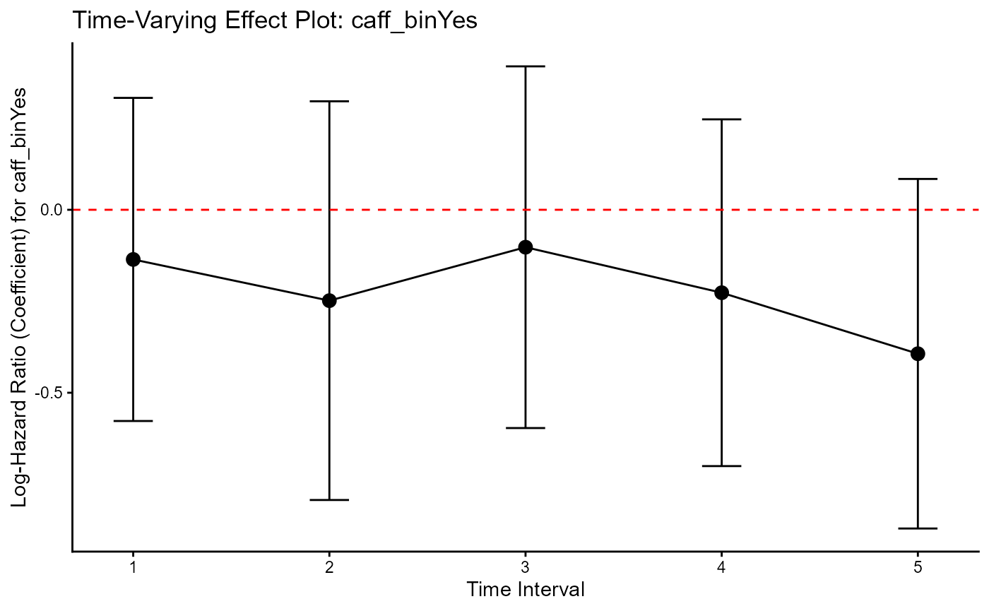

How to Interpret the Results

The output has three key parts: the “Main Model” table, the “Time-Interval” table, and the plot.

Main (Constant Effect) Model: This is the standard, un-split model. It assumes the effect of asthma is constant over time.
Time-Interval Model & Plot: This is the diagnostic test. We check this plot to see if the assumption of the first model was valid.
The plot shows the pooled log-Hazard Ratio (coefficient) for variable of intest across the 5 time intervals. While they are not perfectly flat, the vertical 95% confidence intervals substantially overlap with each other. You could conclude that the constant effect (parallel to proportional hazards) assumption is reasonable. Hence, instead of the time-split model (in the 2nd output), just report the Main (Constant Effect) Model (in the first output).

References

Therneau, Terry, Cindy Crowson, and Elizabeth Atkinson. 2017. “Using Time Dependent Covariates and Time Dependent Coefficients in the Cox Model.” Survival Vignettes 2 (3): 1–25.

1. Visualizing Survey-Weighted Survival Data (svykmplot)