Diagnosing Survey Regression Models with svyTable1

{r setup} knitr::opts_chunk$set( collapse = TRUE, comment = "#>" )

This vignette covers functions in the svyTable1 package for diagnosing fitted survey regression models:

• svydiag(): Checks reliability of regression coefficients.
  
• svygof(): Performs Archer-Lemeshow goodness-of-fit testing for survey logistic models (Archer and Lemeshow 2006).
  
• svyAUC(): Computes design-correct AUC for predictive performance.

These tools provide a structured way to assess whether model coefficients are precise, whether the logistic model fits observed data adequately, and whether predicted probabilities discriminate well between groups.

1. Data and Model Preparation

The examples use complete-case NHANES data from adults aged 20 years or older. A survey-weighted logistic regression model is fitted to predict obesity. This model is used throughout the vignette to illustrate each diagnostic function.

library(svyTable1)
library(survey)
library(dplyr)
library(NHANES)
library(knitr)
library(tidyr)
library(ggplot2)

data(NHANESraw)

nhanes_adults_with_na <- NHANESraw %>%
  filter(Age >= 20) %>%
  mutate(
    ObeseStatus = factor(
      ifelse(BMI >= 30, "Obese", "Not Obese"),
      levels = c("Not Obese", "Obese")
    )
  )

vars_for_complete_table <- c(
  "Age", "Gender", "Race1", "BPSysAve",
  "Pulse", "BMI", "ObeseStatus"
)

nhanes_adults_complete <- nhanes_adults_with_na %>%
  drop_na(all_of(vars_for_complete_table))

adult_design_complete <- svydesign(
  id = ~SDMVPSU,
  strata = ~SDMVSTRA,
  weights = ~WTMEC2YR,
  nest = TRUE,
  data = nhanes_adults_complete
)

fit_obesity <- svyglm(
  ObeseStatus ~ Age + Gender + Race1,
  design = adult_design_complete,
  family = quasibinomial()
)

2. Regression Coefficient Diagnostics (svydiag())

svydiag() produces diagnostics for regression coefficients, including p-values, precision measures, and relative standard errors.

diagnostics_table <- svydiag(fit_obesity)

knitr::kable(
  diagnostics_table,
  caption = "Reliability Diagnostics for NHANES Obesity Model",
  digits = 3
)

Reliability Diagnostics for NHANES Obesity Model

Term	Estimate	SE	p.value	is_significant	CI_Lower	CI_Upper	CI_Width	RSE_percent	is_rse_high
(Intercept)	-0.381	0.109	0.002	TRUE	-0.604	-0.158	0.445	28.486	FALSE
Age	0.008	0.002	0.000	TRUE	0.005	0.012	0.007	20.782	FALSE
Gendermale	-0.061	0.057	0.294	FALSE	-0.179	0.056	0.236	93.470	TRUE
Race1Hispanic	-0.493	0.103	0.000	TRUE	-0.704	-0.282	0.422	20.870	FALSE
Race1Mexican	-0.225	0.087	0.016	TRUE	-0.403	-0.046	0.357	38.733	TRUE
Race1White	-0.654	0.081	0.000	TRUE	-0.821	-0.488	0.334	12.421	FALSE
Race1Other	-1.351	0.131	0.000	TRUE	-1.620	-1.082	0.538	9.707	FALSE

Interpreting the svydiag() Table

• Estimate: Coefficient on the log-odds scale.
  
• p.value, is_significant: Indicate statistical significance.
  
• CI_Width: Reflects the precision of the estimate.
  
• RSE_percent, is_rse_high: Highlight limitations of RSE when estimates are near zero.

3. Goodness-of-Fit Test (svygof())

svygof() implements the Archer and Lemeshow goodness of fit procedure for complex survey logistic regression (Archer and Lemeshow 2006). This test adapts the Hosmer and Lemeshow approach to designs with weights, strata, and clustering.

The function groups respondents by predicted risk and compares observed and expected outcomes while incorporating survey weights. A small p-value provides evidence that predicted risks diverge from observed risks in one or more groups.

This test helps identify lack of fit that may result from omitted interactions or nonlinearities in the model.

gof_results <- svygof(fit_obesity, adult_design_complete)

knitr::kable(
  gof_results,
  caption = "Archer-Lemeshow Goodness-of-Fit Test for Obesity Model"
)

Archer-Lemeshow Goodness-of-Fit Test for Obesity Model

F_statistic	df1	df2	p_value
4.675254	9	24	0.0011839

A significant p-value indicates poor model fit across predicted risk groups.

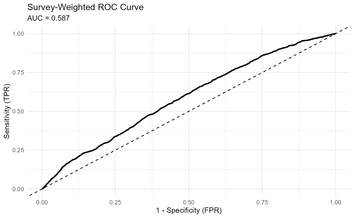
4. Model Performance (svyAUC())

svyAUC() estimates the area under the ROC curve using replicate-weight designs. This produces an AUC estimate and confidence interval that appropriately reflect survey sampling.

The function also returns data for constructing ROC curves. A plot of the ROC curve, along with the AUC estimate, demonstrates how well the model discriminates between obese and non-obese respondents.

A value close to 0.5 indicates little discriminatory value, while higher values indicate stronger predictive performance.

rep_design <- as.svrepdesign(adult_design_complete)

fit_obesity_rep <- svyglm(
  ObeseStatus ~ Age + Gender + Race1,
  design = rep_design,
  family = quasibinomial()
)

auc_results_list <- svyAUC(fit_obesity_rep, rep_design, plot = TRUE)

knitr::kable(
  auc_results_list$summary,
  caption = "Design-Correct AUC for Obesity Model"
)

Design-Correct AUC for Obesity Model

AUC	SE	CI_Lower	CI_Upper
0.5867566	0.0089921	0.569132	0.6043811

ggplot(auc_results_list$roc_data, aes(x = FPR, y = TPR)) +
  geom_line(linewidth = 1) +  # Changed 'size' to 'linewidth'
  geom_abline(linetype = "dashed") +
  labs(
    title = "Survey-Weighted ROC Curve",
    subtitle = paste0("AUC = ", round(auc_results_list$summary$AUC, 3)),
    x = "1 - Specificity (FPR)",
    y = "Sensitivity (TPR)"
  ) +
  theme_minimal()

References

Archer, Kellie J, and Stanley Lemeshow. 2006. “Goodness-of-Fit Test for a Logistic Regression Model Fitted Using Survey Sample Data.” The Stata Journal 6 (1): 97–105.