Chapter 4 Introduction to NHANES
4.1 Instructions
This tutorial is aiming to provide an introduction to NHANES dataset and a guide on how to access the NHANES. It will guide you to retrieve the dataset in two days: CDC website and nhanesA package. At the end of this tutorial, it will cover some basic functions in the nhanesA package.
Accompanying this tutorial is a short Google quiz for your own self-assessment. The instructions of this tutorial will clearly indicate when you should answer which question.
4.2 Learning Objectives
Be familiar with the survey data in NHANES dataset
Be able to import NHANES dataset from CDC website
Be able to set up the nhanesA package and import NHANES dataset from the nhanesA package
Be familiar with the basic functions in the nhanesA package
Be able to understand the difference between NHANES dataset and nhanesA package
4.3 Introduction to NHANES
The National Health and Nutrition Examination Survey (NHANES) is a program with a series of studies aimed at determining the health and nutritional status of Americans, including adults and children. The NHANES program started in the early 1960s and was transformed into a countinuous program in 1999.
Started in the early 1960s, the NHANES programme has consisted of a seriess of surveys concentrating on various population groups or health themes. The survey was transformed into a continuous programme in 1999, with a shifting focus on a variety of health and nutrition measurements. For continuous NHANES,the survey is conducted in two-year cycles, i.e, 1999-2000,2001-2002,etc.
There are 5 types of continues NHANES survey data available to the public:
Demographics Data
Dietary Data
Examination Data
Laboratory Data
Questionnaire Data
We will focus on the continuou NHANES dataset in this series of tutorials. On this CDC website, you will see all the continous NHANES ordered by year.
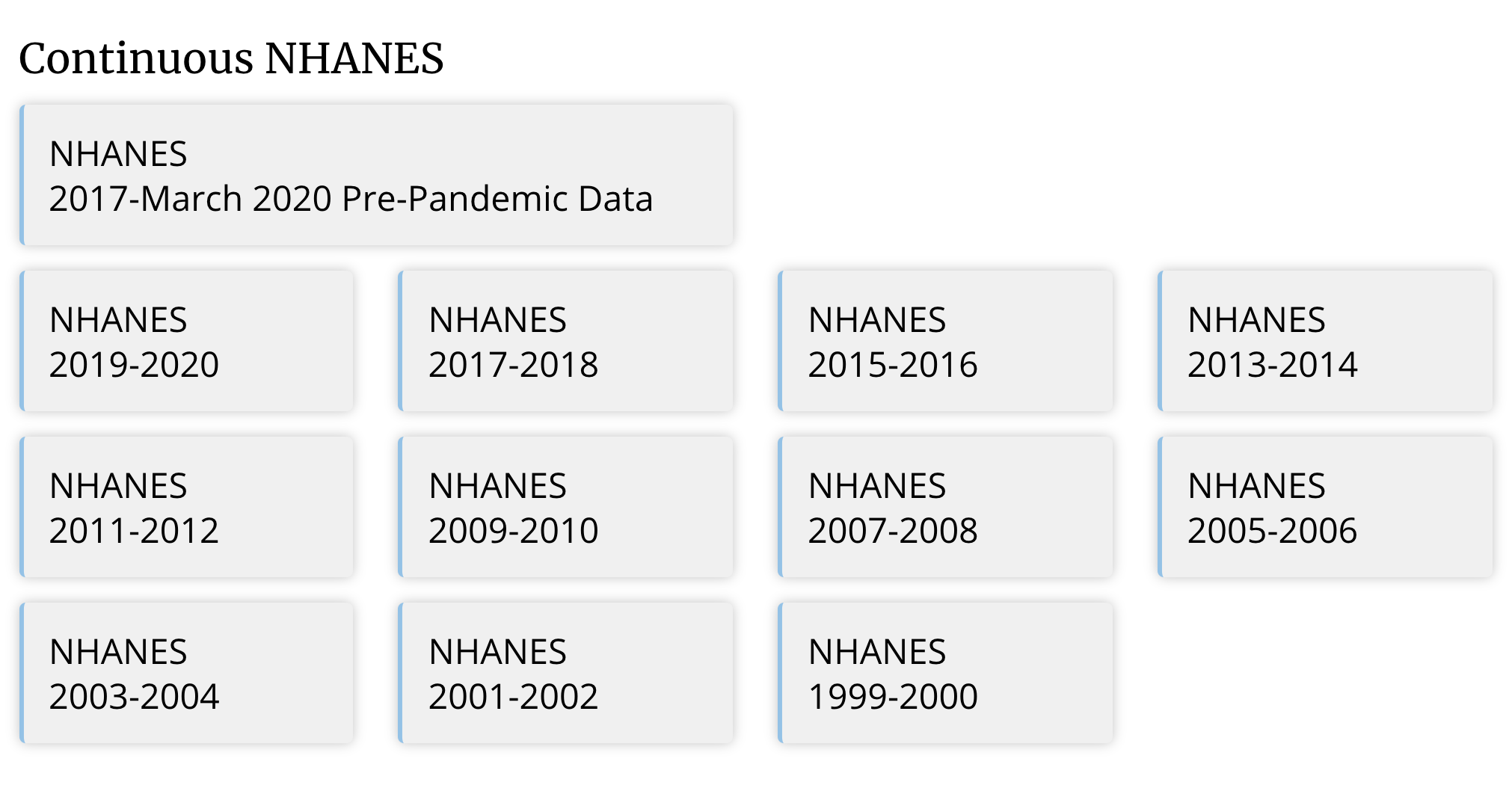
Figure 1. NHANES Datasets from 1999 to 2020
We will use NHANES 2013-2014 just for demostration in this tutorial. If you click on NHANES 2013-2014, you will be directed to the page where you can access the data collected between 2013 and 2014:
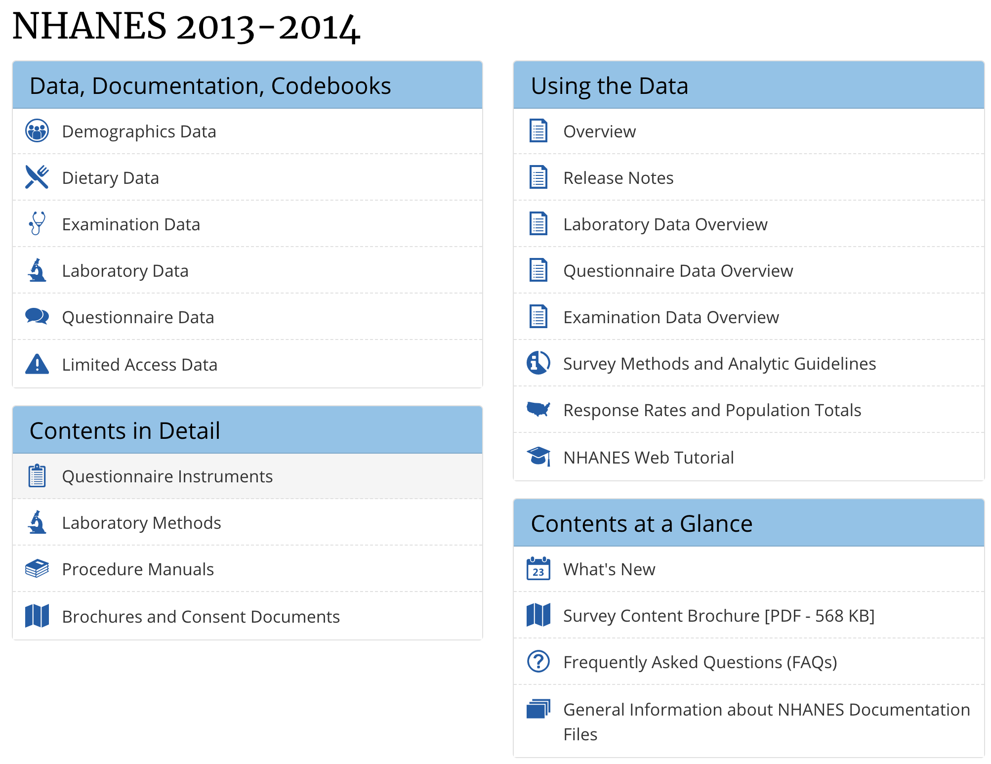
Figure 2. NHANES 2013-2014
We will introduce how to access the data in the following section.
DO QUESTION 1 OF THE QUIZ NOW
- How many categories (available to public) are there in NHANES dataset?
4.4 Importing NHANES dataset from website
Now we will learn how to download the NHANES dataset from CDC website and import it to R. In the last section, we’re on this page and we’ll continue from there.
For example, we want to use the Demographics Data for further analysis. The first step is to download the dataset - click on “Demographics Data”:
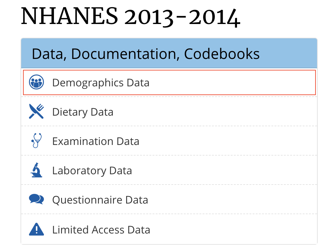
Figure 3. NHANES 2013-2014 Demographics Data
Then, you will see the following page:
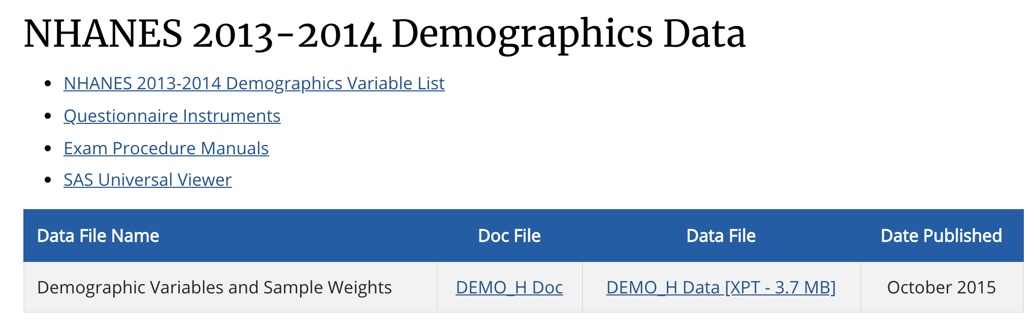
Figure 4. NHANES 2013-2014 Demographics Data
To download the dataset, click on DEMO_H Data [XPT - 3.7 MB] under the Data File.
To find the meanings of the variables, click on NHANES 2013-2014 Demographics Variable List.
Last tutorial, we learned how to import .csv file into R. However, the file we downloaded from CDC website is not a .csv file - it is a .xpt file. Instead of using read_csv(), we need to use read.xport() function housed in SASxport package.
First, we install (if needed) and load theSASxport package:
# install.packages("SASxport")library(SASxport)Then, we are ready to load the datatset into R:
demo <- read.xport("data/DEMO_H.XPT")We can use the head() function to quickly browse the dataset:
head(demo,5)## SEQN SDDSRVYR RIDSTATR RIAGENDR RIDAGEYR RIDAGEMN RIDRETH1 RIDRETH3 RIDEXMON
## 1 73557 8 2 1 69 NA 4 4 1
## 2 73558 8 2 1 54 NA 3 3 1
## 3 73559 8 2 1 72 NA 3 3 2
## 4 73560 8 2 1 9 NA 3 3 1
## 5 73561 8 2 2 73 NA 3 3 1
## RIDEXAGM DMQMILIZ DMQADFC DMDBORN4 DMDCITZN DMDYRSUS DMDEDUC3 DMDEDUC2
## 1 NA 1 1 1 1 NA NA 3
## 2 NA 2 NA 1 1 NA NA 3
## 3 NA 1 1 1 1 NA NA 4
## 4 119 NA NA 1 1 NA 3 NA
## 5 NA 2 NA 1 1 NA NA 5
## DMDMARTL RIDEXPRG SIALANG SIAPROXY SIAINTRP FIALANG FIAPROXY FIAINTRP MIALANG
## 1 4 NA 1 2 2 1 2 2 1
## 2 1 NA 1 2 2 1 2 2 1
## 3 1 NA 1 2 2 1 2 2 1
## 4 NA NA 1 1 2 1 2 2 1
## 5 1 NA 1 2 2 1 2 2 1
## MIAPROXY MIAINTRP AIALANGA DMDHHSIZ DMDFMSIZ DMDHHSZA DMDHHSZB DMDHHSZE
## 1 2 2 1 3 3 0 0 2
## 2 2 2 1 4 4 0 2 0
## 3 2 2 NA 2 2 0 0 2
## 4 2 2 1 4 4 0 2 0
## 5 2 2 NA 2 2 0 0 2
## DMDHRGND DMDHRAGE DMDHRBR4 DMDHREDU DMDHRMAR DMDHSEDU WTINT2YR WTMEC2YR
## 1 1 69 1 3 4 NA 13281.24 13481.04
## 2 1 54 1 3 1 1 23682.06 24471.77
## 3 1 72 1 4 1 3 57214.80 57193.29
## 4 1 33 1 3 1 4 55201.18 55766.51
## 5 1 78 1 5 1 5 63709.67 65541.87
## SDMVPSU SDMVSTRA INDHHIN2 INDFMIN2 INDFMPIR
## 1 1 112 4 4 0.84
## 2 1 108 7 7 1.78
## 3 1 109 10 10 4.51
## 4 2 109 9 9 2.52
## 5 2 116 15 15 5.00Now that we’ve successfully imported the dataset!
Functions debunked
read.xport() is the function we use to read and load SAS XPORT file in R - it is housed in the SASxport package. The arguments are as follows:
read.xport(File Path)
For example: read.xport("../input/demo-h/DEMO_H.XPT")
DO QUESTION 2 OF THE QUIZ NOW
- Which package is read.xport() in?
4.5 Importing NHANES dataset from R package: nhanesA
Another way to access the NHANES dataset is to import it from R packages. One popular R package developed for retrieving NHANES dataset is the nhanesA package.
As introduced before, we need to first install the nhanesA package from CRAN:
# install.packages("nhanesA")Second, we need to load the nhanesA package:
library(nhanesA)Recall that we have 5 data categories available to the public in the NHANES dataset. How do we access the data from nhanesA package?
There is a useful function called - nhanesTables() - list all the data files in each data category in each survey cycle as a table. For example, if we want to see all the Demographics Data in survey cycle 2013-2014:
nhanesTables('DEMO', 2013)## Warning: `xml_nodes()` was deprecated in rvest 1.0.0.
## Please use `html_elements()` instead.## Data.File.Name Data.File.Description
## 1 DEMO_H Demographic Variables and Sample WeightsTo see all the Examination Data in survey cycle 2015-2016:
nhanesTables('EXAM', 2015)## Data.File.Name Data.File.Description
## 1 BPX_I Blood Pressure
## 2 BMX_I Body Measures
## 3 OHXDEN_I Oral Health - Dentition
## 4 OHXREF_I Oral Health - Recommendation of Care
## 5 FLXCLN_I Fluorosis - Clinical
## 6 AUX_I Audiometry
## 7 DXX_I Dual-Energy X-ray Absorptiometry - Whole Body
## 8 AUXAR_I Audiometry - Acoustic Reflex
## 9 AUXTYM_I Audiometry - Tympanometry
## 10 AUXWBR_I Audiometry – Wideband ReflectanceTo see all the Dietary Data in survey cycle 2014-2015:
nhanesTables('DIETARY', 2014)## Data.File.Name
## 1 DR1TOT_H
## 2 DR2TOT_H
## 3 DR1IFF_H
## 4 DR2IFF_H
## 5 DRXFCD_H
## 6 DS1IDS_H
## 7 DSQIDS_H
## 8 DS2IDS_H
## 9 DS1TOT_H
## 10 DS2TOT_H
## 11 DSQTOT_H
## Data.File.Description
## 1 Dietary Interview - Total Nutrient Intakes, First Day
## 2 Dietary Interview - Total Nutrient Intakes, Second Day
## 3 Dietary Interview - Individual Foods, First Day
## 4 Dietary Interview - Individual Foods, Second Day
## 5 Dietary Interview Technical Support File - Food Codes
## 6 Dietary Supplement Use 24-Hour - Individual Dietary Supplements, First Day
## 7 Dietary Supplement Use 30-Day - Individual Dietary Supplements
## 8 Dietary Supplement Use 24-Hour - Individual Dietary Supplements, Second Day
## 9 Dietary Supplement Use 24-Hour - Total Dietary Supplements, First Day
## 10 Dietary Supplement Use 24-Hour - Total Dietary Supplements, Second Day
## 11 Dietary Supplement Use 30-Day - Total Dietary SupplementsFunctions debunked
nhanesTables() is the function we use to display the data in a table format - it is housed in the nhanesA package. The arguments are as follows:
nhanesTables(‘Data Category’, Year)
Note:Abbreviation for the data category in the first argument is listed below:
Demographics Data = DEMO
Dietary Data = DIETARY
Examination Data = EXAM
Labortary Data = LAB
Questionnaire Data = Q
For example: nhanesTables('DEMO', 2013)
For demostration purpose, we will focus on Demographics Data in survey cycle 2013-2014 in the rest of the tutorial.
Now that we need to access and import the dataset from nhanesA package. The nhanes() function (exactly the same as the package name) is used for importing NHANES datasets:
demo <- nhanes('DEMO_H')## Processing SAS dataset DEMO_H ..Browse the top 5 rows in the demo dataframe:
head(demo,5)## SEQN SDDSRVYR RIDSTATR RIAGENDR RIDAGEYR RIDAGEMN RIDRETH1 RIDRETH3 RIDEXMON
## 1 73557 8 2 1 69 NA 4 4 1
## 2 73558 8 2 1 54 NA 3 3 1
## 3 73559 8 2 1 72 NA 3 3 2
## 4 73560 8 2 1 9 NA 3 3 1
## 5 73561 8 2 2 73 NA 3 3 1
## RIDEXAGM DMQMILIZ DMQADFC DMDBORN4 DMDCITZN DMDYRSUS DMDEDUC3 DMDEDUC2
## 1 NA 1 1 1 1 NA NA 3
## 2 NA 2 NA 1 1 NA NA 3
## 3 NA 1 1 1 1 NA NA 4
## 4 119 NA NA 1 1 NA 3 NA
## 5 NA 2 NA 1 1 NA NA 5
## DMDMARTL RIDEXPRG SIALANG SIAPROXY SIAINTRP FIALANG FIAPROXY FIAINTRP MIALANG
## 1 4 NA 1 2 2 1 2 2 1
## 2 1 NA 1 2 2 1 2 2 1
## 3 1 NA 1 2 2 1 2 2 1
## 4 NA NA 1 1 2 1 2 2 1
## 5 1 NA 1 2 2 1 2 2 1
## MIAPROXY MIAINTRP AIALANGA DMDHHSIZ DMDFMSIZ DMDHHSZA DMDHHSZB DMDHHSZE
## 1 2 2 1 3 3 0 0 2
## 2 2 2 1 4 4 0 2 0
## 3 2 2 NA 2 2 0 0 2
## 4 2 2 1 4 4 0 2 0
## 5 2 2 NA 2 2 0 0 2
## DMDHRGND DMDHRAGE DMDHRBR4 DMDHREDU DMDHRMAR DMDHSEDU WTINT2YR WTMEC2YR
## 1 1 69 1 3 4 NA 13281.24 13481.04
## 2 1 54 1 3 1 1 23682.06 24471.77
## 3 1 72 1 4 1 3 57214.80 57193.29
## 4 1 33 1 3 1 4 55201.18 55766.51
## 5 1 78 1 5 1 5 63709.67 65541.87
## SDMVPSU SDMVSTRA INDHHIN2 INDFMIN2 INDFMPIR
## 1 1 112 4 4 0.84
## 2 1 108 7 7 1.78
## 3 1 109 10 10 4.51
## 4 2 109 9 9 2.52
## 5 2 116 15 15 5.00You may get confused why we put DEMO_H instead of DEMO in the argument - recall that DEMO is the abbreviation for Demographcis data. But we also want to tell the function which survey cycle we are particularly interested in.
Go back to the output from nhanesTables(‘DEMO,’ 2013) above, now we have the data file name - DEMO_H and H specifies the survey cycle 2013-2014.
As you are getting familiar with the dataset, you may notice that different letter represents different survey cycle year. For example, H represents survey cycle 2013-2014 and I represents survey cycle 2015-2016.
Functions debunked
nhanes() is the function we use to retrieve the dataset and return a dataframe - it is housed in the nhanesA package. The arguments are as follows:
nhanesTranslate(‘Name of Table’)
For example: nhanes('DEMO_H')
If you run demo alone, you will see that RIAGENDR (gender) is coded as 1 and 2. For ease of future use, we want to translate this 1 and 2 into male and female.
To translate the categorical variables in NHANES, use nhanesTranslate():
demo_translate <- nhanesTranslate('DEMO_H',
                                  c('SEQN', # Respondent sequence number
                                    'RIAGENDR'),
                                 data = demo)
## Warning in FUN(X[[i]], ...): No translation table is available for SEQN## Translated columns: RIAGENDRhead(demo_translate,5)## SEQN SDDSRVYR RIDSTATR RIAGENDR RIDAGEYR RIDAGEMN RIDRETH1 RIDRETH3 RIDEXMON
## 1 73557 8 2 Male 69 NA 4 4 1
## 2 73558 8 2 Male 54 NA 3 3 1
## 3 73559 8 2 Male 72 NA 3 3 2
## 4 73560 8 2 Male 9 NA 3 3 1
## 5 73561 8 2 Female 73 NA 3 3 1
## RIDEXAGM DMQMILIZ DMQADFC DMDBORN4 DMDCITZN DMDYRSUS DMDEDUC3 DMDEDUC2
## 1 NA 1 1 1 1 NA NA 3
## 2 NA 2 NA 1 1 NA NA 3
## 3 NA 1 1 1 1 NA NA 4
## 4 119 NA NA 1 1 NA 3 NA
## 5 NA 2 NA 1 1 NA NA 5
## DMDMARTL RIDEXPRG SIALANG SIAPROXY SIAINTRP FIALANG FIAPROXY FIAINTRP MIALANG
## 1 4 NA 1 2 2 1 2 2 1
## 2 1 NA 1 2 2 1 2 2 1
## 3 1 NA 1 2 2 1 2 2 1
## 4 NA NA 1 1 2 1 2 2 1
## 5 1 NA 1 2 2 1 2 2 1
## MIAPROXY MIAINTRP AIALANGA DMDHHSIZ DMDFMSIZ DMDHHSZA DMDHHSZB DMDHHSZE
## 1 2 2 1 3 3 0 0 2
## 2 2 2 1 4 4 0 2 0
## 3 2 2 NA 2 2 0 0 2
## 4 2 2 1 4 4 0 2 0
## 5 2 2 NA 2 2 0 0 2
## DMDHRGND DMDHRAGE DMDHRBR4 DMDHREDU DMDHRMAR DMDHSEDU WTINT2YR WTMEC2YR
## 1 1 69 1 3 4 NA 13281.24 13481.04
## 2 1 54 1 3 1 1 23682.06 24471.77
## 3 1 72 1 4 1 3 57214.80 57193.29
## 4 1 33 1 3 1 4 55201.18 55766.51
## 5 1 78 1 5 1 5 63709.67 65541.87
## SDMVPSU SDMVSTRA INDHHIN2 INDFMIN2 INDFMPIR
## 1 1 112 4 4 0.84
## 2 1 108 7 7 1.78
## 3 1 109 10 10 4.51
## 4 2 109 9 9 2.52
## 5 2 116 15 15 5.00Functions debunked
nhanesTranslate() is the function we use to translate variables in a dataset - it is housed in the nhanesA package. The arguments are as follows:
nhanesTranslate(‘Name of Dataset’, Columns you want to be translated (can be written as a vector), data = Source Data Frame)
For example: nhanesTranslate('DEMO_H', RIAGENDR, data = demo)
Try it yourself 4.1]4.1
Find all the Examination Data in survey cycle 2013-2014.
Import the blood pressure dataset in the Examination Data in survey cycle 2013-2014
Translate the following variables in the BPX dataset
BPXPULS - Pulse regular or irregular?
BPAARM - Arm selected
DO QUESTIONS 3-5 OF THE QUIZ NOW
Fill in the blank to answer the ‘Try it yourself’ sections:
nhanesTables(
___,___)bpx <- nhanes(
___)bpx_translate <- nhanesTranslate(
___, c(‘BPXPULS,’ ‘BPAARM’), data =___)
4.5.1 Other packages in R
There are other packages that are developed as a tool to retrieve and analyze the NHANES dataset, such as RNHANES package. You are encouraged to explore packages beside nhanesA and play with the data. However, we will be using nhanesA for this series of tutorials, so it is important that you’re familiar with it before we move on.
4.5.2 Alternative ways to download NHANES
If you are wondering how the nhanes() function works, here is a glimpse at what it looks like backstage. First of all, we can create our own function that does the same action as nhanes(). The function we are creating together is not exactly how the nhanes() function works, but the principles are similar. The general gist is that we need a function that can download the .XPT file on the NHANES website and then import it into R as a data frame.
The first step that we need to create a new function is to have a function name and the function… function()! Let’s name our new function downloadnhanes().
downloadnhanes <- function(){
}
Now, our function needs arguments. Let’s give it 2 arguments: the years of the dataset (ex] 2013-2014 or 2014-2015) and the dataset name (ex] DEMO_H or BPX_H).
downloadnhanes <- function(years, prefix_suffix){
}
For the purpose of creating this function step-by-step, let’s say that our years is 2013-2014 and our prefix_suffix is DEMO_H.
years <- '2013-2014'
prefix_suffix <- 'DEMO_H'
Next, our function needs to be able to download the .XPT file straight from the NHANES website. What this means is we need our function to 1. Know where on the web our .XPT file is and 2. Download that file
To do this, we need to create a variable that contains the .XPT’s URL. If we look at the URL of an NHANES dataset’s .XPT file, it should look something along this line: https://wwwn.cdc.gov/nchs/nhanes/2013-2014/DEMO_H.XPT. To lead R to this specific website first before we download the file, we need to use the paste() function like so. Note that “years” and “prefix_suffix” are written as variables because they are two arguments that we would need to define when we use this new function.
url <- paste('https://wwwn.cdc.gov/nchs/nhanes/', years,'/', prefix_suffix, '.XPT', sep = '')Function debunked
paste() is a function we use to combine multiple elements from multiple vectors into one single element. In this case, we are combining hard-wired characters and open variables together into one single url. Some of the main arguments are as follows:
paste(‘Text string that we want to include (note the quotation marks)’, A Defined Variable, sep = ’’ OR ‘/’ OR **’_‘** OR ’&’ etc (this argument tells R how you want each element to be separated, in our case, we don’t want any separator, that’s why there is nothing between the’’ quotation marks))
For example: paste('https://wwwn.cdc.gov/nchs/nhanes/', years,'/', prefix_suffix, '.XPT', sep = '')
After we have our URL, we are ready to download the file! To do this, we use download.file() like so:
download.file(url, tf <- tempfile(), mode = "wb")There are a number of things that you can do with download.file(). We will not go over this function in detail, but here is a helpful website that explains the function really well.
In the function above, we first need the URL of the file that we are downloading - in our case it is just url because we already defined it in the previous paste() function. Next, we want a place to store our downloaded file. In this case, we want it to be tf <- tempfile() because we want to generate a temporary storage space for our downloaded file (you can find more about tempfile() here). After that, we need to use mode = "wb" because our .XPT file is binary. wb is also the most common mode type to use when we use download.file().
Next, we want to import the temporary file tf that we create into R. To do this, we need to use read.xport(). We have already been introduced to the SASxport package, but an alternative to SASxport is foreign. This is another package that deals with importing different data types into R, not just .XPT.
outdf <- foreign::read.xport(tf)Finally, we want to make sure that the file we are importing is a data frame, so we need to use data.frame() for this.
outdf <- data.frame(outdf)Now if we combine everything that we have talked about earlier, our function should look like this:
downloadnhanes <- function(prefix_suffix, years){
    url <- paste('https://wwwn.cdc.gov/nchs/nhanes/', years,'/', prefix_suffix, '.XPT', sep = '')
    download.file(url, tf <- tempfile(), mode = "wb")
    outdf <- foreign::read.xport(tf)
    outdf <- data.frame(outdf)
  return(outdf)
}
Let’s see if it works!
head(
    downloadnhanes('DEMO_H', '2013-2014')
    )
## SEQN SDDSRVYR RIDSTATR RIAGENDR RIDAGEYR RIDAGEMN RIDRETH1 RIDRETH3 RIDEXMON
## 1 73557 8 2 1 69 NA 4 4 1
## 2 73558 8 2 1 54 NA 3 3 1
## 3 73559 8 2 1 72 NA 3 3 2
## 4 73560 8 2 1 9 NA 3 3 1
## 5 73561 8 2 2 73 NA 3 3 1
## 6 73562 8 2 1 56 NA 1 1 1
## RIDEXAGM DMQMILIZ DMQADFC DMDBORN4 DMDCITZN DMDYRSUS DMDEDUC3 DMDEDUC2
## 1 NA 1 1 1 1 NA NA 3
## 2 NA 2 NA 1 1 NA NA 3
## 3 NA 1 1 1 1 NA NA 4
## 4 119 NA NA 1 1 NA 3 NA
## 5 NA 2 NA 1 1 NA NA 5
## 6 NA 1 2 1 1 NA NA 4
## DMDMARTL RIDEXPRG SIALANG SIAPROXY SIAINTRP FIALANG FIAPROXY FIAINTRP MIALANG
## 1 4 NA 1 2 2 1 2 2 1
## 2 1 NA 1 2 2 1 2 2 1
## 3 1 NA 1 2 2 1 2 2 1
## 4 NA NA 1 1 2 1 2 2 1
## 5 1 NA 1 2 2 1 2 2 1
## 6 3 NA 1 2 2 1 2 2 1
## MIAPROXY MIAINTRP AIALANGA DMDHHSIZ DMDFMSIZ DMDHHSZA DMDHHSZB DMDHHSZE
## 1 2 2 1 3 3 0 0 2
## 2 2 2 1 4 4 0 2 0
## 3 2 2 NA 2 2 0 0 2
## 4 2 2 1 4 4 0 2 0
## 5 2 2 NA 2 2 0 0 2
## 6 2 2 1 1 1 0 0 0
## DMDHRGND DMDHRAGE DMDHRBR4 DMDHREDU DMDHRMAR DMDHSEDU WTINT2YR WTMEC2YR
## 1 1 69 1 3 4 NA 13281.24 13481.04
## 2 1 54 1 3 1 1 23682.06 24471.77
## 3 1 72 1 4 1 3 57214.80 57193.29
## 4 1 33 1 3 1 4 55201.18 55766.51
## 5 1 78 1 5 1 5 63709.67 65541.87
## 6 1 56 1 4 3 NA 24978.14 25344.99
## SDMVPSU SDMVSTRA INDHHIN2 INDFMIN2 INDFMPIR
## 1 1 112 4 4 0.84
## 2 1 108 7 7 1.78
## 3 1 109 10 10 4.51
## 4 2 109 9 9 2.52
## 5 2 116 15 15 5.00
## 6 1 111 9 9 4.79It works! But does it match with the output of our usual nhanes() function? Let’s test it out.
head(
    nhanes('DEMO_H')
    )
## Processing SAS dataset DEMO_H ..## SEQN SDDSRVYR RIDSTATR RIAGENDR RIDAGEYR RIDAGEMN RIDRETH1 RIDRETH3 RIDEXMON
## 1 73557 8 2 1 69 NA 4 4 1
## 2 73558 8 2 1 54 NA 3 3 1
## 3 73559 8 2 1 72 NA 3 3 2
## 4 73560 8 2 1 9 NA 3 3 1
## 5 73561 8 2 2 73 NA 3 3 1
## 6 73562 8 2 1 56 NA 1 1 1
## RIDEXAGM DMQMILIZ DMQADFC DMDBORN4 DMDCITZN DMDYRSUS DMDEDUC3 DMDEDUC2
## 1 NA 1 1 1 1 NA NA 3
## 2 NA 2 NA 1 1 NA NA 3
## 3 NA 1 1 1 1 NA NA 4
## 4 119 NA NA 1 1 NA 3 NA
## 5 NA 2 NA 1 1 NA NA 5
## 6 NA 1 2 1 1 NA NA 4
## DMDMARTL RIDEXPRG SIALANG SIAPROXY SIAINTRP FIALANG FIAPROXY FIAINTRP MIALANG
## 1 4 NA 1 2 2 1 2 2 1
## 2 1 NA 1 2 2 1 2 2 1
## 3 1 NA 1 2 2 1 2 2 1
## 4 NA NA 1 1 2 1 2 2 1
## 5 1 NA 1 2 2 1 2 2 1
## 6 3 NA 1 2 2 1 2 2 1
## MIAPROXY MIAINTRP AIALANGA DMDHHSIZ DMDFMSIZ DMDHHSZA DMDHHSZB DMDHHSZE
## 1 2 2 1 3 3 0 0 2
## 2 2 2 1 4 4 0 2 0
## 3 2 2 NA 2 2 0 0 2
## 4 2 2 1 4 4 0 2 0
## 5 2 2 NA 2 2 0 0 2
## 6 2 2 1 1 1 0 0 0
## DMDHRGND DMDHRAGE DMDHRBR4 DMDHREDU DMDHRMAR DMDHSEDU WTINT2YR WTMEC2YR
## 1 1 69 1 3 4 NA 13281.24 13481.04
## 2 1 54 1 3 1 1 23682.06 24471.77
## 3 1 72 1 4 1 3 57214.80 57193.29
## 4 1 33 1 3 1 4 55201.18 55766.51
## 5 1 78 1 5 1 5 63709.67 65541.87
## 6 1 56 1 4 3 NA 24978.14 25344.99
## SDMVPSU SDMVSTRA INDHHIN2 INDFMIN2 INDFMPIR
## 1 1 112 4 4 0.84
## 2 1 108 7 7 1.78
## 3 1 109 10 10 4.51
## 4 2 109 9 9 2.52
## 5 2 116 15 15 5.00
## 6 1 111 9 9 4.79The two imported datasets are identical! Fantastic, our new function works! And that’s just a sneak peak of what goes behind our nhanes() function.
The function that we went over in this tutorial is originally found on the CDC website. For simplification and educational purposes, the function has been simplified. You can find the original function here.
4.6 Summary and Takeaways
By the end of this tutorial, you should be able to know what is NHANES and how to retrieve the NHANES dataset. You should also be familiar with the functions housed in nhanesA mentioned in this tutorial.
For the next two tutorials, we will introduce two new packages - dplyr for data analysis and ggplot for data visulization. We will continusely use NHANES dataset for illustration and you’ll likely be using NHANES dataset for your own research in the future. Make sure you’re familiar with NHANES dataset before we move on.