2  Propensity score

Propensity Score Analysis

Propensity score analysis is a method for adjusting for confounding in observational studies by balancing treatment or exposure groups based on the probability of receiving treatment, using investigator-specified measured covariates.

2.1 Propensity Score Analysis

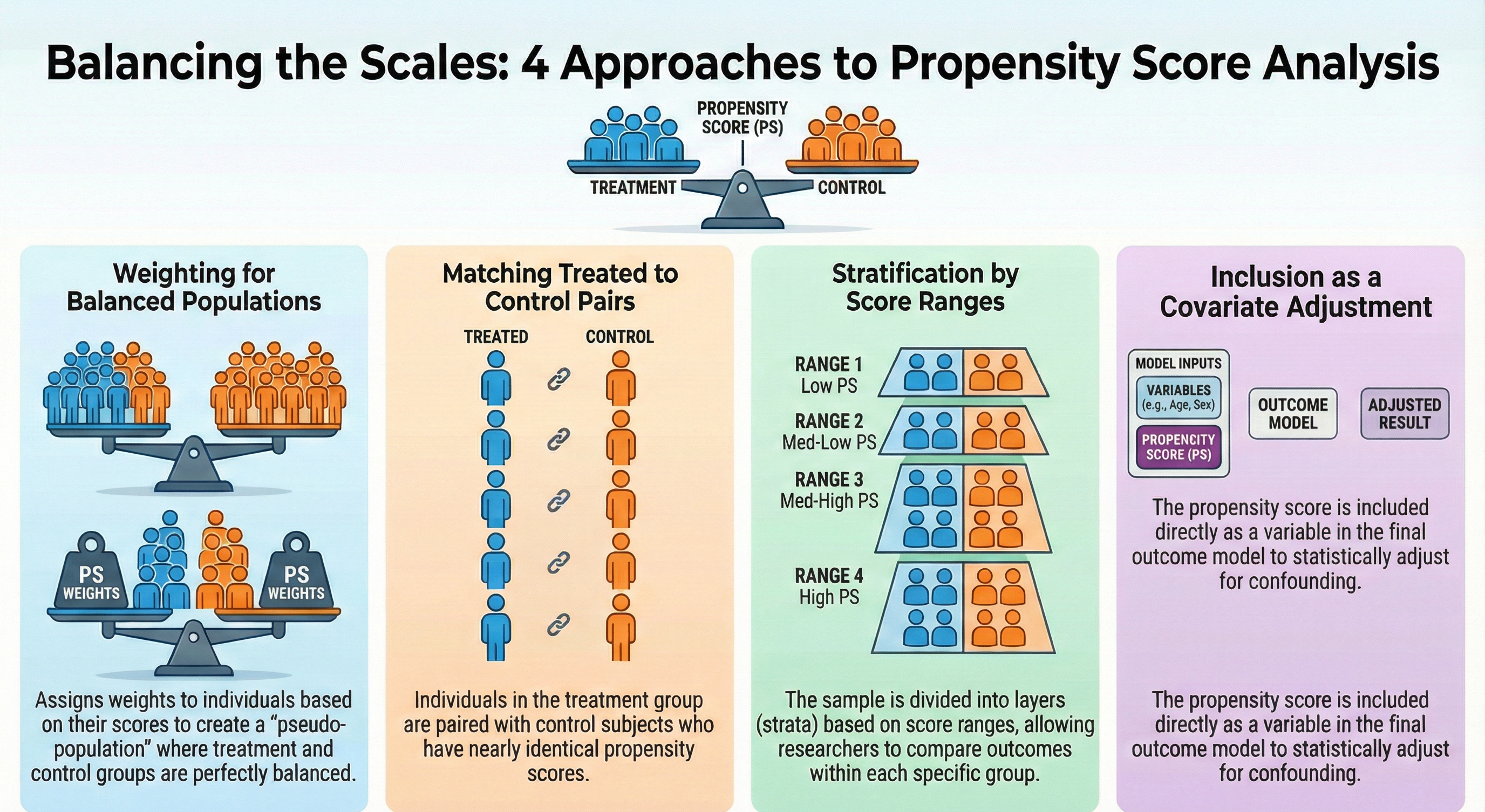
There are four approaches to propensity score (PS) analysis:

1. Weighting: Assign weights to individuals based on their propensity scores to create a pseudo-population where treatment groups are balanced.
2. Matching: Match individuals in the treatment group with individuals in the control group based on their propensity scores.
3. Stratification: Divide the sample into strata based on the propensity score and compare outcomes within each stratum.
4. Covariate Adjustment: Include the propensity score as a covariate in a outcome model to adjust for confounding.

2.2 Propensity Score Weighting

Austin and Stuart (2015)

For this demonstration, we will focus on the Weighting approach. The other approaches are not covered in this demonstration, but they can be implemented using similar steps as shown below.

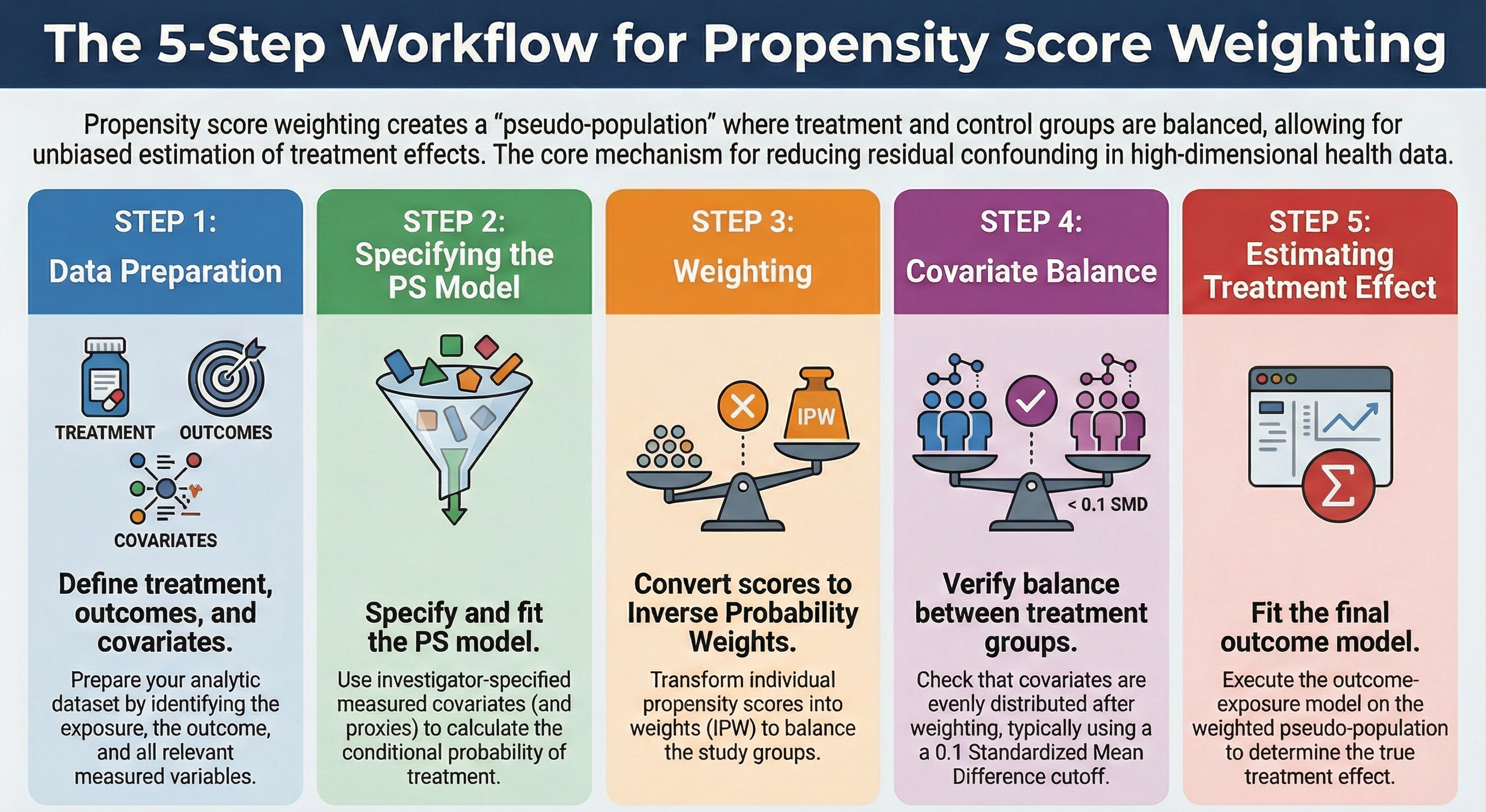
There are four steps in propensity score weighting (after data preparation):

0. Data preparation: Prepare the data by creating the treatment/exposure, outcome, and covariates.
1. Specifying PS & fit model: Specify the propensity score model with investigator-specified measured covariates and fit the model
2. Weighting: Convert PS to inverse probability weights (IPW).
3. Covariate balance: Check the balance of covariates between treatment groups after weighting.
4. Estimating treatment effect: Fit the outcome model on the pseudo population.

2.2.1 Step 0: Data preparation

2.2.1.1 Creating Analytic data

3 cycles of NHANES datasets were - downloaded from the US CDC website - recoded for consistency, and - merged together to make an analytic data.

Details of data download process, and recoding and merging are discussed in Appendix.

flowchart LR
  A[NHANES] --> C1(2013-2014 cycle) --> ss1(10,175<br>participants)
  A --> C2(2015-2016 cycle) --> ss2(9,971<br>participants)
  A --> C3(2017-2018 cycle) --> ss3(9,254<br>participants)

  ss(7,585<br>participants<br>after imposing<br>eligibility criteria)

  ss1 --> ss
  ss2 --> ss
  ss3 --> ss

  %% 1. Define a reusable style class named 'customOrange'
  classDef customOrange fill:#FFA500,color:#333,stroke:#A66C00

  %% 2. Apply the class to the desired nodes
  class A,C1,C2,C3,ss1,ss2,ss3,ss customOrange;

Our study population was restricted to the U.S. population who were

• 20 years or older and
• not pregnant at the time of survey data collection, and
• who had available International Classification of Diseases (ICD) codes to ensure we can extract sufficient proxy information for the analysis (discussed in step 1).

To simplify the analysis, we only considered complete case data.

Important

This table compares our treated and untreated groups before any statistical adjustment.

It answers the question: ‘Are these two groups comparable at the start?’

• In observational studies (unlike randomized trials), these groups are often very different.
• We use the Standardized Mean Difference (SMD) to measure imbalance.
  • Unlike p-values, SMD is independent of sample size, making it a reliable metric for comparing group differences regardless of how large our dataset is.
  • If you see variables with an SMD > 0.1, these are variables that differ between our groups. These imbalances act as confounders that could bias our results if we don’t adjust for them.

# Table 1
library(tableone)
tab1 <- CreateTableOne(vars = investigator.specified.covariates, 
                       strata = "exposure",
                       data = hdps.data, 
                       test = FALSE)
print(tab1, 
      showAllLevels = TRUE, 
      noSpaces = TRUE, 
      quote = FALSE, 
      smd = TRUE, 
      printToggle = FALSE) |>
  kbl(caption = "Table 1: Baseline Characteristics by Exposure Group") |>
  kable_styling(bootstrap_options = c("striped", "hover", "condensed"), 
                full_width = FALSE)

Table 1: Baseline Characteristics by Exposure Group

	level	0	1	SMD
n		2223	1616
age.cat (%)	20-49	703 (31.6)	528 (32.7)	0.149
	50-64	673 (30.3)	579 (35.8)
	65+	847 (38.1)	509 (31.5)
sex (%)	Male	1009 (45.4)	648 (40.1)	0.107
	Female	1214 (54.6)	968 (59.9)
education (%)	Less than high school	322 (14.5)	248 (15.3)	0.242
	High school	951 (42.8)	860 (53.2)
	College graduate or above	950 (42.7)	508 (31.4)
race (%)	White	933 (42.0)	677 (41.9)	0.452
	Black	302 (13.6)	367 (22.7)
	Hispanic	453 (20.4)	424 (26.2)
	Others	535 (24.1)	148 (9.2)
marital (%)	Never married	274 (12.3)	196 (12.1)	0.115
	Married/with partner	1432 (64.4)	964 (59.7)
	Other	517 (23.3)	456 (28.2)
income (%)	less than $20,000	364 (16.4)	300 (18.6)	0.184
	$20,000 to $74,999	984 (44.3)	821 (50.8)
	$75,000 and Over	875 (39.4)	495 (30.6)
born (%)	Born in US	1342 (60.4)	1170 (72.4)	0.257
	Other place	881 (39.6)	446 (27.6)
year (%)	NHANES 2013-2014 public release	1026 (46.2)	703 (43.5)	0.090
	NHANES 2015-2016 public release	305 (13.7)	195 (12.1)
	NHANES 2017-2018 public release	892 (40.1)	718 (44.4)
diabetes.family.history (%)	No	1900 (85.5)	1251 (77.4)	0.208
	Yes	323 (14.5)	365 (22.6)
medical.access (%)	No	150 (6.7)	71 (4.4)	0.103
	Yes	2073 (93.3)	1545 (95.6)
smoking (%)	Never smoker	1350 (60.7)	943 (58.4)	0.095
	Previous smoker	576 (25.9)	484 (30.0)
	Current smoker	297 (13.4)	189 (11.7)
diet.healthy (%)	Poor or fair	436 (19.6)	615 (38.1)	0.487
	Good	904 (40.7)	650 (40.2)
	Very good or excellent	883 (39.7)	351 (21.7)
physical.activity (%)	No	1901 (85.5)	1317 (81.5)	0.108
	Yes	322 (14.5)	299 (18.5)
sleep (mean (SD))		7.40 (1.48)	7.30 (1.60)	0.067
uric.acid (mean (SD))		5.25 (1.38)	5.81 (1.53)	0.383
protein.total (mean (SD))		7.08 (0.46)	7.06 (0.45)	0.049
bilirubin.total (mean (SD))		0.58 (0.29)	0.52 (0.33)	0.193
phosphorus (mean (SD))		3.74 (0.55)	3.68 (0.58)	0.109
sodium (mean (SD))		139.83 (2.62)	139.74 (2.74)	0.031
potassium (mean (SD))		4.05 (0.39)	4.07 (0.39)	0.046
globulin (mean (SD))		2.87 (0.46)	3.00 (0.46)	0.289
calcium.total (mean (SD))		9.41 (0.39)	9.34 (0.40)	0.166
systolicBP (mean (SD))		126.07 (19.52)	129.23 (17.72)	0.169
diastolicBP (mean (SD))		70.17 (11.59)	72.35 (11.82)	0.186
high.cholesterol (%)	No	1137 (51.1)	756 (46.8)	0.087
	Yes	1086 (48.9)	860 (53.2)

2.2.2 Step 1: Specifying PS & fit model

We build the propensity score model in this data using the investigator-specified covariates.

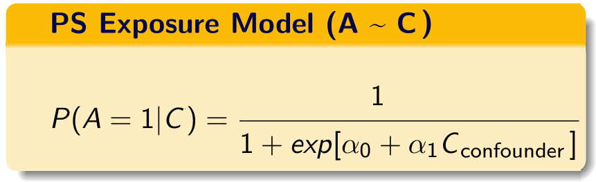
C = investigator-specified covariates.

If you are somewhat unfamiliar with propensity score paradigm, look at tutorials dedicated towards that topic. There are additional tutorials also talking about propensity score weighting.

2.2.2.1 PS model specification

Now let us create the propensity score formula with the investigator-specified covariates:

covform <- paste0(investigator.specified.covariates, collapse = "+")
ps.formula <- as.formula(paste0("exposure", "~", covform))
ps.formula
#> exposure ~ age.cat + sex + education + race + marital + income + 
#>     born + year + diabetes.family.history + medical.access + 
#>     smoking + diet.healthy + physical.activity + sleep + uric.acid + 
#>     protein.total + bilirubin.total + phosphorus + sodium + potassium + 
#>     globulin + calcium.total + systolicBP + diastolicBP + high.cholesterol

• Only use *investigator specified covariates** to build the formula.
• During the construction of the propensity score model, researchers should consider incorporating additional model specifications, such as interactions and polynomials, if they are deemed necessary.

2.2.2.2 Fit the PS model

require(WeightIt)
W.out <- weightit(ps.formula, 
                    data = hdps.data, 
                    estimand = "ATE",
                    method = "ps")

• Use that formula to estimate propensity scores.
• In this demonstration, we did not use stabilize = TRUE. However, stabilized propensity score weights often reduce the variance of treatment effect estimates.

2.2.2.3 Obtain PS

hdps.data$ps <- W.out$ps
ggplot(hdps.data, aes(x = ps, fill = factor(exposure))) +
  geom_density(alpha = 0.5) +
  scale_fill_manual(values = c("darkblue", "darkred")) +
  theme_classic()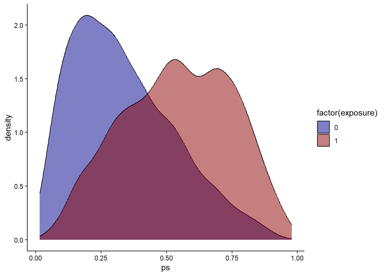

Check propensity score overlap in both exposure groups.

2.2.3 Step 2: Weighting

As mentioned, we only talk about inverse probability weighting in our current context.

The specific formula used to calculate the weights depends on the estimand of interest. Let \(A\) be the binary treatment indicator (\(A=1\) for treated, \(A=0\) for control) and \(e\) be the estimated propensity score.

Average Treatment Effect (ATE): (this is what we are using here) The goal is to estimate the effect if the entire population were treated versus if the entire population were untreated. \[w_{ATE} = \frac{A}{e} + \frac{1-A}{1-e}\]

Average Treatment Effect on the Treated (ATT): The goal is to estimate the effect specifically for those who actually received the treatment. \[w_{ATT} = A + \frac{e(1-A)}{1-e}\]

hdps.data$w <- W.out$weights
summary(hdps.data$w)
#>    Min. 1st Qu.  Median    Mean 3rd Qu.    Max. 
#>   1.016   1.277   1.559   2.008   2.144  45.795

ggplot(hdps.data, aes(x = "", y = w)) +
  geom_boxplot(fill = "lightblue", 
               color = "blue", 
               size = 1) +
  geom_text(aes(x = 1, y = max(w), 
                label = paste0("Max = ", round(max(w), 2))), 
            vjust = 1.5, 
            hjust = -0.3, 
            size = 4, 
            color = "red") +
  geom_text(aes(x = 1, y = min(w), 
                label = paste0("Min = ", round(min(w), 2))), 
            vjust = -2.5, 
            hjust = -0.3, 
            size = 4, 
            color = "red") +
  ggtitle("Boxplot of Inverse Probability Weights") +
  xlab("") +
  ylab("Weights") +
  theme_classic()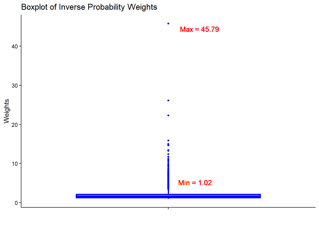

• Check the summary statistics of the weights to assess whether there are extreme weights. Less extreme weights now?

2.2.4 Step 3: Covariate balance

require(cobalt)
love.plot(x = W.out,
          thresholds = c(m = .1), 
          var.order = "unadjusted",
          stars = "raw")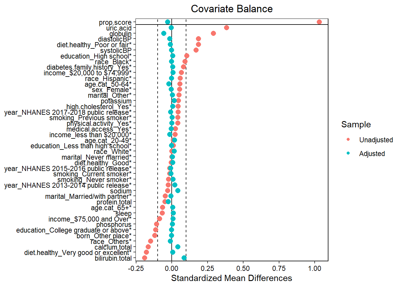

• Assess balance against SMD 0.1. Still balanced?
• Predictive measures such as c-statistics are not helpful in this context (Westreich et al. 2011): “use of the c-statistic as a guide in constructing propensity scores may result in less overlap in propensity scores between treated and untreated subjects”!

Warning

You balance the groups without looking at the outcome (blinded). You only proceed to the outcome analysis once you have achieved balance (SMD < 0.1). This mimics a Randomized Controlled Trial (RCT).

# Extract balance statistics including SMD
bal_stats <- bal.tab(W.out, 
                     stats = c("m", "v"), # 'm' for mean diff (SMD), 'v' for variance ratios
                     thresholds = c(m = 0.1)) # Highlight SMDs > 0.1

# Display the balance table as a nice kable
bal_stats$Balance %>%
  select(Diff.Adj) %>% # Select only the adjusted (weighted) SMD column
  arrange(desc(abs(Diff.Adj))) %>% # Sort by absolute SMD to see worst imbalance first
  kbl(caption = "Standardized Mean Differences (SMD) After Weighting",
      digits = 3) %>%
  kable_styling(bootstrap_options = c("striped", "hover", "condensed"), 
                full_width = FALSE)

Standardized Mean Differences (SMD) After Weighting

	Diff.Adj
bilirubin.total	0.085
globulin	-0.058
calcium.total	0.041
sodium	0.040
prop.score	-0.030
protein.total	-0.026
age.cat_50-64	-0.022
year_NHANES 2013-2014 public release	0.019
age.cat_20-49	0.017
potassium	0.017
income_less than $20,000	-0.016
race_White	0.016
diastolicBP	-0.015
diet.healthy_Poor or fair	-0.012
race_Others	-0.011
year_NHANES 2015-2016 public release	-0.010
year_NHANES 2017-2018 public release	-0.010
sleep	0.009
income_$20,000 to $74,999	0.008
income_$75,000 and Over	0.008
smoking_Current smoker	-0.008
marital_Married/with partner	-0.007
smoking_Never smoker	0.007
education_High school	0.006
diet.healthy_Very good or excellent	0.006
uric.acid	-0.006
medical.access_Yes	-0.006
diet.healthy_Good	0.006
sex_Female	-0.005
diabetes.family.history_Yes	0.005
high.cholesterol_Yes	0.005
age.cat_65+	0.005
marital_Never married	0.004
education_College graduate or above	-0.004
phosphorus	0.004
systolicBP	-0.003
race_Black	-0.003
marital_Other	0.003
born_Other place	-0.003
education_Less than high school	-0.003
race_Hispanic	-0.002
physical.activity_Yes	-0.002
smoking_Previous smoker	0.001

2.2.5 Step 4: Estimating treatment effect

2.2.5.1 Set outcome formula

out.formula <- as.formula(paste0("outcome", "~", "exposure"))
out.formula
#> outcome ~ exposure

We are again using a crude weighted outcome model here.

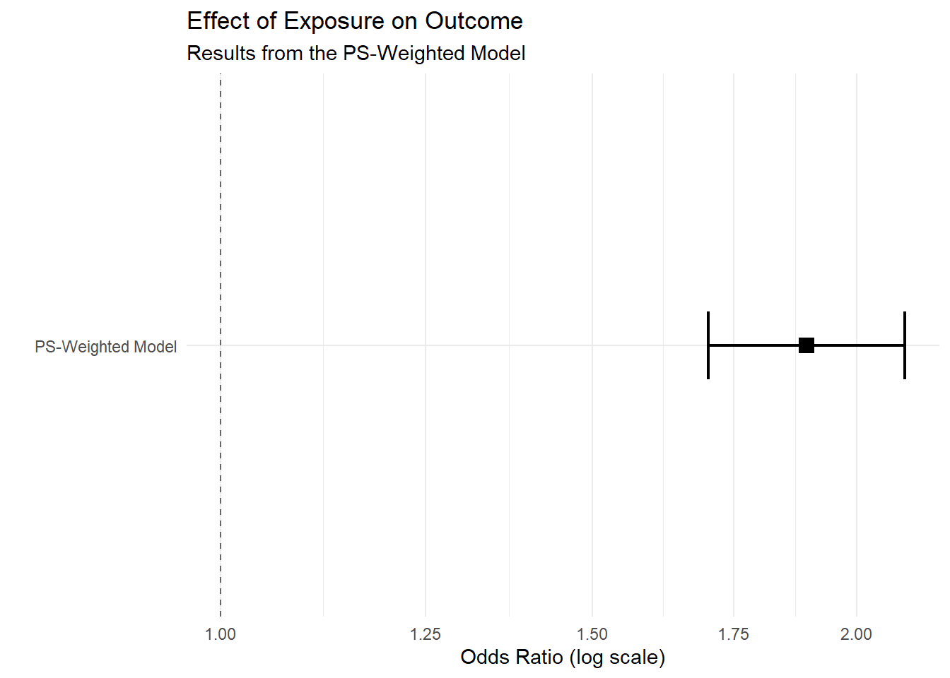
2.2.5.2 Obtain OR

fit <- glm(out.formula,
            data = hdps.data,
            weights = W.out$weights,
            family= binomial(link = "logit"))
fit.summary <- summary(fit)$coef["exposure",
                                 c("Estimate", 
                                   "Std. Error", 
                                   "Pr(>|z|)")]
fit.summary[2] <- sqrt(sandwich::sandwich(fit)[2,2])
require(lmtest)
conf.int <- confint(fit, "exposure", level = 0.95, method = "hc1")

fit.summary_with_ci.ps <- c(fit.summary, conf.int)
knitr::kable(t(round(fit.summary_with_ci.ps,2))) 

Estimate	Std. Error	Pr(>|z|)	2.5 %	97.5 %
0.64	0.1	0	0.53	0.75

2.2.5.3 Obtain RD

fit <- glm(out.formula,
            data = hdps.data,
            weights = W.out$weights,
            family= gaussian(link = "identity"))
fit.summary <- summary(fit)$coef["exposure",
                                 c("Estimate", 
                                   "Std. Error", 
                                   "Pr(>|t|)")]
fit.summary[2] <- sqrt(sandwich::sandwich(fit)[2,2])
require(lmtest)
conf.int <- confint(fit, "exposure", level = 0.95, method = "hc1")
fit.summary_with_ci.ps.rd <- c(fit.summary, conf.int)
knitr::kable(t(round(fit.summary_with_ci.ps.rd,2))) 

Estimate	Std. Error	Pr(>|t|)	2.5 %	97.5 %
0.11	0.02	0	0.09	0.14

2.3 Summary of Causal Inference Methods

Method Category	Specific Methods	Advantages	Limitations
Regression & Outcome Modeling	Regression, G-Computation, Decision Trees, Random Forest	• Efficiency: High statistical efficiency (small SEs) if correctly specified. • Flexibility (ML): ML versions handle non-linearities/interactions automatically.	• Model Dependence: Biased if outcome model is misspecified. • No Design Phase: Risk of “p-hacking” as analysis is not blinded to outcome. • Inference: Standard SEs/CIs often invalid for pure ML methods.
Propensity Score (Exposure Modeling)	PS Matching, PS Weighting	• Design Separation: Balances groups blind to outcome (mimics RCT). • Dimension Reduction: Summarizes confounders into one score. • Diagnostics: Forces check of “common support” (overlap).	• Overfitting: High-dimensional data can lead to perfect prediction and extreme weights. • Instability: Sensitive to lack of overlap (positivity violations). • Precision: Less efficient than correct regression.
Double Robust Methods	Augmented IPW, TMLE, Double ML, Causal Forest	• Double Robustness: Unbiased if either outcome or exposure model is correct. • Valid Inference with ML: Allows use of ML for variable selection with valid CIs/SEs.	• Complexity: Computationally intensive and harder to implement/interpret. • Positivity Sensitivity: Can still be unstable with severe overlap issues.
Instrumental Variable Methods	2SLS	• Unmeasured Confounding: Can account for unmeasured confounders (unlike all others above).	• Assumption Heavy: Valid instruments are extremely rare in observational health data. • Efficiency: Large standard errors compared to other methods.

Shared Limitations

A critical limitation shared by both regression and propensity score-based methods is their reliance on the exchangeability assumption; both frameworks can only account for measured variables included in the model. Consequently, even with advanced adjustment (e.g., Double Robust Methods), these methods remain inherently subject to unmeasured confounding bias if essential risk factors or common causes are omitted from the data.

Austin, Peter C, and Elizabeth A Stuart. 2015. “Moving Towards Best Practice When Using Inverse Probability of Treatment Weighting (IPTW) Using the Propensity Score to Estimate Causal Treatment Effects in Observational Studies.” Statistics in Medicine 34 (28): 3661–79.

Westreich, Daniel, Stephen R Cole, Michele Jonsson Funk, M Alan Brookhart, and Til Stürmer. 2011. “The Role of the c-Statistic in Variable Selection for Propensity Score Models.” Pharmacoepidemiology and Drug Safety 20 (3): 317–20.