1 Data to Analyze

To answer the research question “Does obesity increase the risk of developing diabetes?” in the U.S. context, we do the following:

1.1 Choose a U.S. data source

Data source: National Health and Nutrition Examination Survey (NHANES) (Disease Control and Prevention 2021)
- 2013-2014,
- 2015-2016,
- 2017-2018
Availability: NHANES is a publicly available dataset that can be downloaded for free from the CDC website.
Design: Observational cross-sectional data. Hence, inferring causality is not a possibility or our objective here.

1.2 Confounder identification

Directed acyclic graph (DAG)

(Greenland, Pearl, and Robins 1999)

flowchart TB
  A[Obesity A] --> Y(Diabetes Y)
  L[Confounders C] --> Y
  L --> A

Hypothesized Directed acyclic graph drawn based on analyst’s best understanding of the literature

Variable Selection Strategy

In standard Propensity Score analysis, we rely on Investigator-Specified Covariates. According to causal theory, we should include:

✅ Confounders: Variables causing both Exposure and Outcome.
✅ Risk Factors: Variables causing the Outcome (to improve precision)

We must avoid:

❌ Instruments: Variables causing Exposure only (increases variance/bias).
❌ Colliders: Effects of both Exposure and Outcome (induces bias).

Measured vs. unmeasured

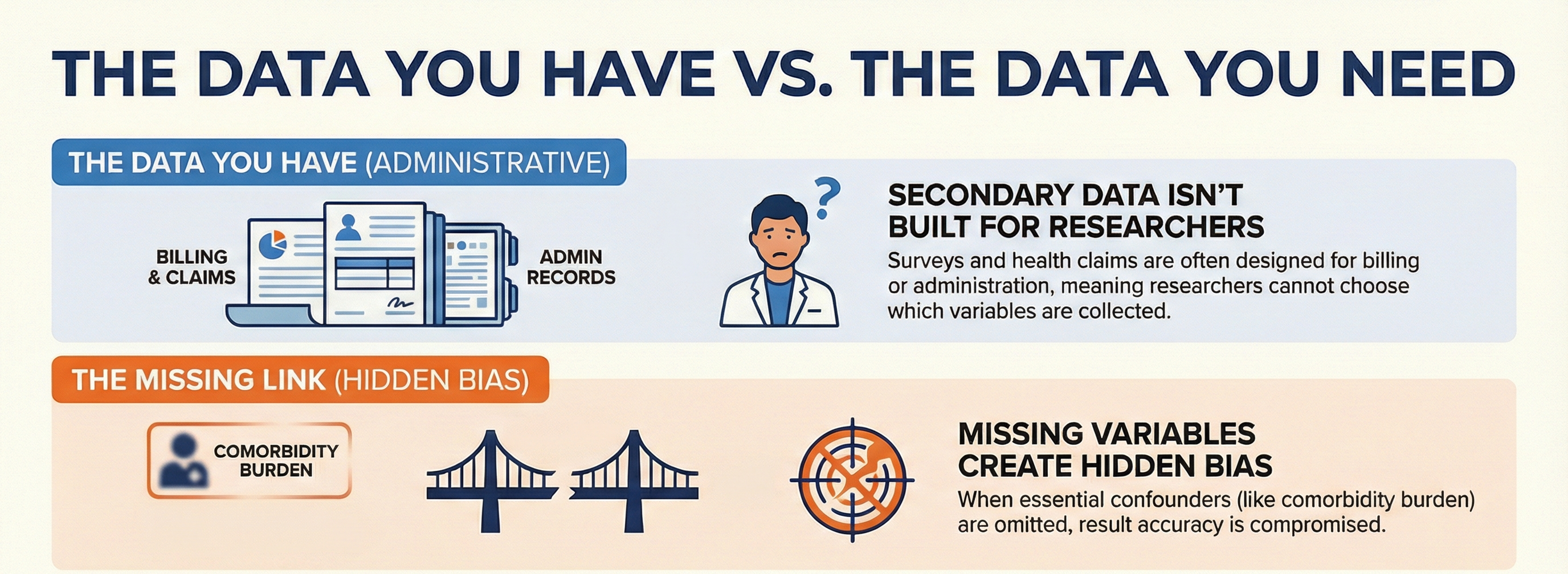
When using secondary data sources such as NHANES or health administrative databases, the data is often collected for administrative, billing or general monitoring rather than specific research questions. Because researchers do not have control over which variables are included in the survey/questionnaire, essential variables required to fully adjust for bias (confounders) may be missing.

Exposure: Being obese

Outcome: Developing diabetes

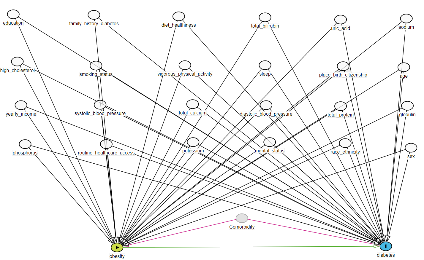
Confounders: Demographic and lab variables

1.3 Structure of the data

flowchart LR
  D[NHANES 2013-14] --> demo[Demographic Variables and Sample Weights]
  demo --> Age
  demo --> Sex
  demo --> Education
  demo --> r[Race or ethnicity]
  demo --> m[Marital status]
  demo --> Income
  demo --> b[Birth place]
  demo --> sf[Survey features: sampling weights, strata, cluster]
  D --> bmi[Body Measures]
  bmi --> Obesity
  D --> diq[Diabetes]
  diq --> Diabetes
  diq --> f[Family history of diabetes]
  D --> smq[Smoking - Cigarette Use]
  smq --> Smoking
  D --> dbq[Diet Behavior & Nutrition]
  dbq --> Diet
  D --> paq[Physical Activity]
  paq --> p[Physical activities]
  D --> huq[Hospital Utilization & Access to Care]
  huq --> mm[Medical access]
  D --> bpx[Blood Pressure]
  bpx --> sbp[Systolic Blood Pressure]
  bpx --> dbp[Diastolic Blood Pressure]
  D --> bpq[Blood Pressure & Cholesterol]
  bpq --> hc[High cholesterol]
  D --> slq[Sleep Disorders]
  slq --> Sleep
  D --> biopro[Standard Biochemistry Profile]
  biopro --> u[Uric acid]
  biopro --> Protein
  biopro --> Bilirubin
  biopro --> Phosphorus
  biopro --> Sodium
  biopro --> Potassium
  biopro --> Globulin
  biopro --> Calcium
  D --> rxq[Prescription Medications - ICD-10-CM codes]
  style D fill:#FFA500;
  style rxq fill:#00FF00;
  style biopro fill:#00FF00;
  style slq fill:#00FF00;
  style bpq fill:#00FF00;
  style bpx fill:#00FF00;
  style huq fill:#00FF00;
  style paq fill:#00FF00;
  style dbq fill:#00FF00;
  style smq fill:#00FF00;
  style diq fill:#00FF00;
  style bmi fill:#00FF00;
  style demo fill:#00FF00;

We do the same for the following cycles:

NHANES 2015-16
NHANES 2017-18

1.4 Identify measured and unmeasured variables in the data

Find variables capturing the following concepts in the data based on a hypothesized DAG.

Role	Data Component	Variables considered based on DAG
Outcome	DIQ	Have diabetes¹
Exposure	BMX	Obese; BMI >= 30
Confounder	(demographic) DEMO	Age, Sex, Education, Race/ethnicity, Marital status, Annual household income, County of birth, Survey cycle year
	(behaviour) SMQ, PAQ, SLQ, DBQ	Smoking², Vigorous work activity, Sleep³, Diet⁴
	(health history / access) DIQ, HUQ	Diabetes family history, Access to care⁵
	(lab) BPX, BPQ, BIOPRO	Blood pressure (systolic, diastolic⁶), Cholesterol, Uric acid, Total Protein, Total Bilirubin, Phosphorus, Sodium, Potassium, Globulin, Total Calcium

14 demographic, behavioral, health history related variables
- Mostly categorical
11 lab variables
- Mostly continuous

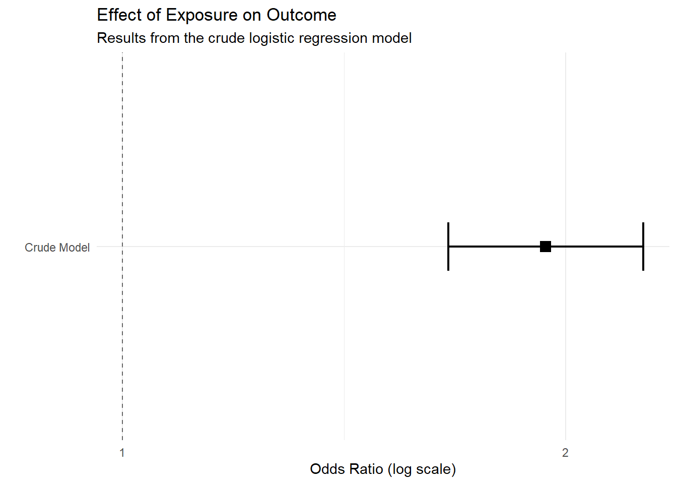
1.5 Fitting crude model to obtain OR

Crude association

Here we estimate the crude association between the exposure and the outcome.

out.formula <- as.formula("outcome ~ exposure")
fit <- glm(out.formula,
            data = hdps.data,
            family= binomial(link = "logit"))
fit.summary <- summary(fit)$coef["exposure",
                                 c("Estimate", 
                                   "Std. Error", 
                                   "Pr(>|z|)")]
fit.ci <- confint(fit, level = 0.95)["exposure", ]
fit.summary_with_ci.crude <- c(fit.summary, fit.ci)
knitr::kable(t(round(fit.summary_with_ci.crude, 2)))

Estimate	Std. Error	Pr(>\|z\|)	2.5 %	97.5 %
0.66	0.08	0	0.51	0.81

combination of (a) Doctor told you have diabetes, (b) Taking insulin now, (c) Take diabetic pills to lower blood sugar.↩︎
cigarette use (at least 100 cigarettes in life)↩︎
Sleep hours/workdays↩︎
How healthy is the diet↩︎
Routine place to go for healthcare↩︎
average of 4 measurements↩︎