Binary outcomes: right-heart catheterization • dr3

Everything in dr3 works the same way for a binary outcome; only the scale of the answer changes — the average treatment effect becomes a risk difference, E[Y^1] - E[Y^0] on the probability scale. We use the right-heart catheterization (RHC) study of Connors et al. (1996): does placing a Swan-Ganz catheter within 24h of ICU admission (swang1) change 30-day mortality? It is a real observational dataset, so there is no known truth.

Load the data

dr_rhc() downloads RHC from the public Vanderbilt biostatistics repository via Hmisc::getHdata() — dr3 ships no data — and returns the treatment, the binary outcome, and one-hot-encoded covariates.

str(rhc[c("name", "outcome_type")])
#> List of 2
#>  $ name        : chr "RHC (right heart cath -> dth30)"
#>  $ outcome_type: chr "binary (mortality risk difference)"
c(n = length(rhc$Y), treated = sum(rhc$A), deaths = sum(rhc$Y))
#>       n treated  deaths 
#>    5735    2184    1918

One call

dr_panel() detects the binary outcome and targets on the risk-difference scale automatically (the TMLE scaling uses y_range = c(0, 1)). Pass family_y = binomial() so the shared Super Learner fits the outcome model as a probability.

fit <- dr_panel(rhc$Y, rhc$A, rhc$X, family_y = binomial(),
                SL.library = c("SL.mean", "SL.glm", "SL.glmnet"), seed = 1)
#> Loading required package: nnls
#> Loading required namespace: glmnet
#> Warning in predict.lm(object, newdata, se.fit, scale = 1, type = if (type == :
#> prediction from rank-deficient fit; attr(*, "non-estim") has doubtful cases
#> Warning in predict.lm(object, newdata, se.fit, scale = 1, type = if (type == :
#> prediction from rank-deficient fit; attr(*, "non-estim") has doubtful cases
#> Warning in predict.lm(object, newdata, se.fit, scale = 1, type = if (type == :
#> prediction from rank-deficient fit; attr(*, "non-estim") has doubtful cases
#> Warning in predict.lm(object, newdata, se.fit, scale = 1, type = if (type == :
#> prediction from rank-deficient fit; attr(*, "non-estim") has doubtful cases
#> Warning in predict.lm(object, newdata, se.fit, scale = 1, type = if (type == :
#> prediction from rank-deficient fit; attr(*, "non-estim") has doubtful cases
#> Warning in predict.lm(object, newdata, se.fit, scale = 1, type = if (type == :
#> prediction from rank-deficient fit; attr(*, "non-estim") has doubtful cases
fit
#> dr3 estimator panel  (n = 5735)
#>       estimator         nuisance estimate         95% CI
#>   g-computation             full    0.050               
#>            IPTW             full    0.055               
#>            AIPW             full    0.055 (0.028, 0.081)
#>            TMLE             full    0.056 (0.029, 0.082)
#>      AIPW = DML        cross-fit    0.056 (0.029, 0.084)
#>  TMLE (CV-TMLE)        cross-fit    0.058 (0.030, 0.085)
#>  AIPW (DC-AIPW) double-cross-fit    0.054 (0.029, 0.080)
#>  TMLE (DC-TMLE) double-cross-fit    0.058 (0.033, 0.084)

plot(fit, xlab = "risk difference (30-day mortality)")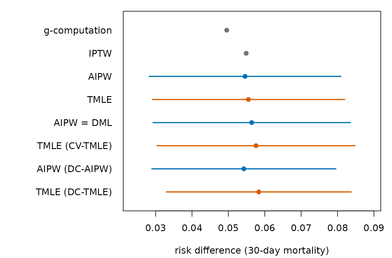

Reading the panel

Every doubly-robust estimate is positive — RHC is associated with higher 30-day mortality — reproducing the direction of the original Connors et al. finding. As in the continuous case, the full-sample AIPW sits a little below the cross-fit estimates (in-sample overfitting under-sizes its one-step correction), and cross-fitting (DML, CV-TMLE) restores it. The singly-robust plug-ins (g-computation, IPTW) carry no analytic interval.

Because the outcome is a 0/1 event, the estimates and their Wald intervals are on the risk-difference scale: a value of 0.05 means five extra deaths per hundred patients attributable to catheterization under the no-unmeasured-confounding assumption.