12 Sensitivity Analyses

This chapter presents several analyses conducted to further assess and understand the primary findings regarding association between early-smoking initiation and mortality. It includes two sensitivity analyses and one exploratory analysis of a potential mediator.

Adjustment for Socioeconomic Status (SES) Proxies: This analysis investigates whether the observed associations are substantially influenced by socioeconomic factors. This is achieved by adjusting for additional variables, such as family poverty income ratio (PIR), which compares household income to the poverty threshold adjusted for household size and composition (NHANES variable INDFMPIR) , and the education level of the household head (NHANES variable DMDHREDU). These variables serve as proxies for family socioeconomic status.
Effect Modification by Race/Ethnicity (2011-2018): This analysis examines how findings might vary when considering the “non-Hispanic Asian” racial classification, which was introduced in the 2011 survey cycle. It focuses on effect modification by race/ethnicity within the survey cycles spanning 2011 to 2018, which incorporate the Asian race/ethnicity category.
Exploratory Analysis of Smoking Duration: This analysis investigates the relationship between the age of smoking initiation and the total duration of smoking, a potential mediator in the pathway to mortality.

The key methods and the paper figures/tables they reproduce are summarized below:

Analysis	Purpose	Key Method	Reproduces
Adjustment for SES Proxies	To test if the main findings are robust to confounding by socioeconomic status.	Added `pir` (income) and `HHedu` (education) as covariates to the adjusted Cox model.	Appendix Figure 5
Effect Modification by Race (2011-2018)	To specifically investigate the association within the non-Hispanic Asian population.	Subset the data to the 2011-2018 cycles and included the `race2` variable (with the ‘Asian’ category) in the effect modification model.	Appendix Table 3 and Appendix Figure 4
Smoking Duration	Explore if earlier initiation is linked to longer smoking duration.	Create boxplots of smoking duration stratified by initiation age.	Appendix Figures 1-3

Show/Hide Code

# Load required packages
library(readr)
library(car)
library(plyr)
library(dplyr)
library(DataExplorer)
library(tableone)
library(Publish)
library(survey)
options(survey.want.obsolete=TRUE)
library(survival)
require(knitr)
require(kableExtra)
require(stringr) 
library(ggplot2) 
library(expss) 
library(readxl) 
library(patchwork)
library(forcats)
library(nhanesA)

12.1 Sensitivity Analysis 1: Adjustment for SES Proxies

12.1.1 Data Reprocessing with SES Variables

Our primary analysis did not include socioeconomic status (SES) variables because they had a high number of missing values. To ensure these factors were not confounding our results, we performed this sensitivity analysis. This required reprocessing the raw NHANES data to create a new dataset that includes the following 2 variables as well:

Demographics:

“INDFMPIR”: Ratio of family income to poverty (family SES)
“DMDHREDU”: Education level of the household head (family SES)

R Code Chunk 1: Data Reprocessing and Cleaning with SES Variables

The code steps for data downloading, cleaning, and merging are nearly identical to the process in main analysis. The key new data preparation steps for this sensitivity analysis are the cleaning of the two SES proxy variables, pir and HHedu.

Show/Hide Code

# File Names
demo <- c("DEMO", "DEMO_B", "DEMO_C", "DEMO_D", "DEMO_E", 
          "DEMO_F", "DEMO_G", "DEMO_H", "DEMO_I", "DEMO_J")
smoking <- c("SMQ", "SMQ_B", "SMQ_C", "SMQ_D", "SMQ_E",
             "SMQ_F", "SMQ_G", "SMQ_H", "SMQ_I", "SMQ_J")

# 10 Data Files
demo_data_files <- readRDS("data/demo_data_files.rds")
smoking_data_files <- readRDS("data/smoking_data_files.rds")

# Set Columns
demo_columns <- c( "SEQN", "RIDAGEYR", "RIAGENDR", "RIDRETH1",
                   "INDFMPIR", "DMDHREDU", "DMDHREDZ", # *** these are new
                   "DMDBORN", "DMDBORN2", "DMDBORN4", "SDDSRVYR", 
                   "WTINT2YR", "WTMEC2YR", "SDMVPSU", "SDMVSTRA")
smoking_columns <- c("SEQN", "SMQ020", "SMD030", "SMQ040", "SMD055")


# DEMOGRAPHICS
demo_data_files_2 <- lapply(seq_along(demo_data_files), function(i) 
  {
  current_cycle_data <- demo_data_files[[i]]
  original <- demo[i] 
  
  # Select Columns
  subset_data <- current_cycle_data %>% 
    dplyr::select(dplyr::any_of(demo_columns))
  # Translate 
  translated_data <- nhanesTranslate(original,
                                     names(subset_data), 
                                     data = subset_data)
  # Return
  return(translated_data) 
})
#> Translated columns: RIAGENDR RIDRETH1 DMDHREDU DMDBORN SDDSRVYR
#> Translated columns: RIAGENDR RIDRETH1 DMDHREDU DMDBORN SDDSRVYR
#> Translated columns: RIAGENDR RIDRETH1 DMDHREDU DMDBORN SDDSRVYR
#> Translated columns: RIAGENDR RIDRETH1 DMDHREDU DMDBORN SDDSRVYR
#> Translated columns: RIAGENDR RIDRETH1 DMDHREDU DMDBORN2 SDDSRVYR
#> Translated columns: RIAGENDR RIDRETH1 DMDHREDU DMDBORN2 SDDSRVYR
#> Translated columns: RIAGENDR RIDRETH1 DMDHREDU DMDBORN4 SDDSRVYR
#> Translated columns: RIAGENDR RIDRETH1 DMDHREDU DMDBORN4 SDDSRVYR
#> Translated columns: RIAGENDR RIDRETH1 DMDHREDU DMDBORN4 SDDSRVYR
#> Translated columns: RIAGENDR RIDRETH1 DMDHREDZ DMDBORN4 SDDSRVYR


# SMOKING
smoking_data_files_2 <- lapply(seq_along(smoking_data_files), function(i) 
  {
  current_cycle_data <- smoking_data_files[[i]]
  original <- smoking[i]

  # Select Columns
  subset_data <- current_cycle_data %>%
    dplyr::select(dplyr::any_of(smoking_columns))
  # Translate
  translated_data <- nhanesTranslate(original, 
                                     names(subset_data), 
                                     data = subset_data)
  # Return
  return(translated_data)
})
#> Translated columns: SMQ020 SMQ040
#> Translated columns: SMQ020 SMQ040
#> Translated columns: SMQ020 SMQ040
#> Translated columns: SMQ020 SMQ040
#> Translated columns: SMQ020 SMQ040
#> Translated columns: SMQ020 SMQ040
#> Translated columns: SMQ020 SMQ040
#> Translated columns: SMQ020 SMQ040
#> Translated columns: SMQ020 SMQ040
#> Translated columns: SMQ020 SMQ040


# MERGE
data_all <- lapply(seq_along(demo_data_files_2), function(i) {
  demo_df <- demo_data_files_2[[i]]
  smoking_df <- smoking_data_files_2[[i]]
  
  # Merge by SEQN
  merged_df <- join_all(list(demo_df, smoking_df), 
                        by = "SEQN", 
                        type = 'full')
  return(merged_df)
})


# Rename 
data_all2 <- data_all
for (i in seq_along(data_all2)) {
  df <- as.data.frame(data_all2[[i]])

  if ("DMDBORN2" %in% names(df)) {
    names(df)[names(df) == "DMDBORN2"] <- "DMDBORN"
  } else if ("DMDBORN4" %in% names(df)) {
    names(df)[names(df) == "DMDBORN4"] <- "DMDBORN"
  }
  data_all2[[i]] <- df
}

Show/Hide Code


for (i in seq_along(data_all2)) {
  # Set Data
  dat2 <- data_all2[[i]]
  
  ## ID
  dat2$id <- dat2$SEQN
  
  ## Demographic
    ### Age (for eligibility)
  dat2$age <- dat2$RIDAGEYR
  
    ### Sex
  dat2$sex <- dat2$RIAGENDR
  
    ### Race/Ethnicity
  dat2$race <- dat2$RIDRETH1
  dat2$race <- car::recode(dat2$race, recodes = "
    'Non-Hispanic White'='White';
    'Non-Hispanic Black'='Black';
    c('Mexican American','Other Hispanic')='Hispanic';
    else='Others'")
  dat2$race <- factor(dat2$race, 
                      levels = c("White", "Black", "Hispanic", "Others"))
  
    ### Country of birth
  dat2$born <- dat2$DMDBORN
  dat2$born <- car::recode(dat2$born, recodes = "
    c('Born in Mexico','Born Elsewhere', 'Others') = 'Other place';
    c('Born in 50 US States or Washington, DC', 'Born in 50 US states or Washington, DC') = 'Born in US';
    else = NA")
  dat2$born <- factor(dat2$born, 
                      levels = c("Born in US", "Other place"))
  
  data_all2[[i]] <- dat2
}

Poverty Income Ratio: The poverty income ratio (INDFMPIR) is provided as a continuous variable. To make it easier to use in our models, the following code uses the cut() function to categorize the numeric ratio into five distinct, interpretable groups, from “Below Poverty Line” to “High Income.”

Show/Hide Code

for (i in seq_along(data_all2)) {
  # Set Data
  dat2 <- data_all2[[i]]
  
  # Set Poverty Income Ratio
  dat2$pir <- dat2$INDFMPIR
  
  # Cut into five distinct groups
  dat2$pir <- cut(dat2$pir,
                  breaks = c(-Inf, 1, 1.99, 3.99, 4.99, Inf),
                  labels = c("Below Poverty Line",
                             "Near Poverty Line",
                             "Low to Middle Income",
                             "Middle to High Income",
                             "High Income"),
                  right = FALSE)
  
  # Return
  data_all2[[i]] <- dat2
}

Household Head Education Level: The coding for household head education also changes over the survey years, with the 2017-2018 cycle using a different variable name (DMDHREDZ) and different text labels. The code below uses an if-else statement to handle this inconsistency. It applies one set of recoding rules for the first nine cycles and a different set for the final 2017-2018 cycle, ensuring the final HHedu variable is harmonized across all datasets.

Show/Hide Code

for (i in seq_along(data_all2)) {
  # Set Data
  dat2 <- data_all2[[i]]
  if (i < 10) {
  
  # Set Education Level of the Household Head
  # Now, use case_when() for robust recoding
  dat2$HHedu <- case_when(
    dat2$DMDHREDU %in% c("Less Than 9th Grade", "9-11th Grade (Includes 12th grade with no diploma)", "Less than high school degree") ~ "Less than high school",
    dat2$DMDHREDU %in% c("High School Grad/GED or equivalent", "Some College or AA degree", "High school grad/GED or some col") ~ "High school or college",
    dat2$DMDHREDU == "College Graduate or above" ~ "College graduate or above",
    TRUE ~ NA_character_ # This handles "Refused", "Don't know", and any other non-matches
    )
  
  # Convert to a factor with the correct levels
  dat2$HHedu <- factor(dat2$HHedu, levels = c('Less than high school',
                                              'High school or college', 
                                              'College graduate or above'))
  # Return
  data_all2[[i]] <- dat2
  }
  
  # For the 10th dataset (2017-2018)
  else { 
    dat2$HHedu <- as.character(dat2$DMDHREDZ)
    dat2$HHedu <- dplyr::recode(dat2$HHedu,
                         `Less than high school degree` = 'Less than high school',
                         `High school grad/GED or some college/AA degree` = 'High school or college',
                         `College graduate or above` = 'College graduate or above',
                         .default = NA_character_ 
                         #`Refused` = NA_character_,
                         #`Don't know` = NA_character_
                         )
    dat2$HHedu <- factor(dat2$HHedu, levels = c('Less than high school',
                                                'High school or college',
                                                'College graduate or above'))
    
    # Return
    data_all2[[i]] <- dat2
    }
}

Show/Hide Code

# Remaining Variables

for (i in seq_along(data_all2)) {
  # Set Data
  dat2 <- data_all2[[i]]
  ## Smoking
    ### Status
  dat2$smoking <- dat2$SMQ020
  dat2$smoking <- car::recode(dat2$smoking, " 'Yes' = 'Current smoker'; 'No' = 'Never smoker'; else=NA  ")
  dat2$smoking <- factor(dat2$smoking, levels = c("Never smoker", "Previous smoker", "Current smoker"))
  dat2$smoking[dat2$SMQ040 == "Not at all?" | dat2$SMQ040 == "Not at all"] <- "Previous smoker"
  
    ### Age smoking started
  dat2$smoking.age <- dat2$SMD030
  dat2$smoking.age[dat2$smoking.age == 777] <- NA
  dat2$smoking.age[dat2$smoking.age == 999] <- NA
  dat2$smoking.age[dat2$smoking == "Never smoker"] <- 99 # 99 means never smoker
  
    ### Whether smoking started age of 15 or before
  dat2$smoked.while.child <- car::recode(dat2$smoking.age, " 0 = 'No'; 1:15 = 'Yes'; else = NA ", as.factor = T)
  
  ## Survey features
    ### Weight
  dat2$survey.weight <- dat2$WTINT2YR #WTMEC2YR # MEC weights
  
    ### PSU 
  dat2$psu <- as.factor(dat2$SDMVPSU)
  
    ### Strata
  dat2$strata <- as.factor(dat2$SDMVSTRA)
  
  ## Survey year
  dat2$year <- dat2$SDDSRVYR
  
  data_all2[[i]] <- dat2
}

NOTE: The following code chunk recodes the variable, SMD055, which stands for the age cigarettes were last smoked regularly. This variable is not available for the cycle 2017-2018, thus it is set as NA. This part is essential for the plots in section 12.3 Appendix B: Exploratory Analysis of Smoking Duration below.

Show/Hide Code

for (i in seq_along(data_all2)) {
  # Set Data
  dat2 <- data_all2[[i]]
  if (i < 10) {
    ### Age smoking quit
    dat2$smoking.quit.age <- dat2$SMD055
    dat2$smoking.quit.age[dat2$smoking.quit.age == 777] <- NA
    dat2$smoking.quit.age[dat2$smoking.quit.age == 999] <- NA
  }
  else {
    dat2$smoking.quit.age <- NA
  }
  data_all2[[i]] <- dat2
}

R Code Chunk 2: Save New Files

After the same remaining data processing steps are taken, theses 10 new files are also saved with the selected variables saved in vars.

Show/Hide Code

nhanes_all <- c("nhanes00", "nhanes01", "nhanes03", "nhanes05", 
                "nhanes07", "nhanes09", "nhanes11", 
                "nhanes13", "nhanes15", "nhanes17")

vars <- c("id", "age", "sex", "race", "born", "pir", "HHedu", 
          "smoking.age", "smoking.quit.age",
          "smoked.while.child", "smoking",
          "survey.weight", "psu", "strata", "year")


cycle_years <- c("1999-2000", "2001-2002", "2003-2004", "2005-2006", "2007-2008", 
                 "2009-2010", "2011-2012", "2013-2014", "2015-2016", "2017-2018")

for (i in seq_along(data_all2)) {
  dat2 <- data_all2[[i]]
  
  nhanes_i <- nhanes_all[i]
  assign(nhanes_i, dat2[, vars], envir = .GlobalEnv)
  
  analytic <- subset(get(nhanes_i), age >= 20)
  cat("Processing:", nhanes_i, "\n")
  print(dim(analytic))
  
  analytic_i <- paste0("analytic", substr(nhanes_i, 7, 8))
  assign(analytic_i, analytic, envir = .GlobalEnv)
  
  # Create 'data2' directory if it does not exist
  if (!dir.exists("data2")) {
    dir.create("data2")
  }

  # Save
  save(list = c(nhanes_i, analytic_i),
       file = file.path("data2", paste0(analytic_i, ".RData")))
}

# Bind all
dat.full <- rbind(nhanes00, nhanes01, nhanes03,
                  nhanes05, nhanes07, nhanes09,
                  nhanes11, nhanes13, nhanes15, 
                  nhanes17)

# Corrected weights
dat.full$survey.weight.new <- dat.full$survey.weight/length(unique(dat.full$year))
dat.full$survey.weight <- NULL
names(dat.full)
dim(dat.full)

Show/Hide Code

# Mortality Data
mort2000 <- readRDS(file = "data/Mortalitydata/mort2000.RData")
mort2001 <- readRDS(file = "data/Mortalitydata/mort2001.RData")
mort2003 <- readRDS(file = "data/Mortalitydata/mort2003.RData")
mort2005 <- readRDS(file = "data/Mortalitydata/mort2005.RData")
mort2007 <- readRDS(file = "data/Mortalitydata/mort2007.RData")
mort2009 <- readRDS(file = "data/Mortalitydata/mort2009.RData")
mort2011 <- readRDS(file = "data/Mortalitydata/mort2011.RData")
mort2013 <- readRDS(file = "data/Mortalitydata/mort2013.RData")
mort2015 <- readRDS(file = "data/Mortalitydata/mort2015.RData")
mort2017 <- readRDS(file = "data/Mortalitydata/mort2017.RData")

# Merge
dat.mortality <- rbind(mort2000, mort2001, mort2003,
                       mort2005, mort2007, mort2009, 
                       mort2011, mort2013, mort2015, 
                       mort2017)
table(dat.mortality$mort_eligstat, useNA = "always")

# Merging analytic and mortality data
dat.full.with.mortality <- merge(dat.full, dat.mortality, by = "id", all.x = TRUE)
dim(dat.full.with.mortality)

Show/Hide Code

# Recoding
dat.full.with.mortality$exposure.cat <- car::recode(dat.full.with.mortality$smoking.age, " 
                                                    c(0,99) = 'Never smoked'; 
                                                    1:9 = 'Started before 10';
                                                    10:14 = 'Started at 10-14';
                                                    15:17 = 'Started at 15-17';
                                                    18:20 = 'Started at 18-20';
                                                    21:80 = 'Started after 20';
                                                    else = NA ", 
                                                    as.factor = TRUE)
dat.full.with.mortality$exposure.cat <- factor(dat.full.with.mortality$exposure.cat, 
                                               levels = c("Never smoked",
                                                          'Started before 10',
                                                          'Started at 10-14',
                                                          "Started at 15-17",
                                                          "Started at 18-20",
                                                          "Started after 20"))

# Survival time - Person-Months of Follow-up from NHANES Interview date
# changed to "Number of Person Months of Follow-up from NHANES Mobile Examination Center (MEC) date" from "Number of Person Months of Follow-up from NHANES interview date" as we are using MCQ data (not really changed it again!)
dat.full.with.mortality$stime.since.interview <- dat.full.with.mortality$mort_permth_int # mort_permth_exm 
summary(dat.full.with.mortality$stime.since.interview) 
#>    Min. 1st Qu.  Median    Mean 3rd Qu.    Max.    NA's 
#>     0.0    59.0   113.0   117.9   172.0   250.0   42252

# Age in month
dat.full.with.mortality$age.month <- dat.full.with.mortality$age * 12
summary(dat.full.with.mortality$age.month)
#>    Min. 1st Qu.  Median    Mean 3rd Qu.    Max. 
#>     0.0   120.0   288.0   373.5   624.0  1020.0

# Survival time - Person-Months of Follow-up from birth = birth to screening + screening to event/censor
dat.full.with.mortality$stime.since.birth <- with(dat.full.with.mortality, age.month + stime.since.interview)
# converted back to year so that KM plot is in years / HR results remain the same (added)
dat.full.with.mortality$stime.since.birth <- dat.full.with.mortality$stime.since.birth/12
dat.full.with.mortality$stime.since.birth[is.na(dat.full.with.mortality$stime.since.interview)] <- NA
summary(dat.full.with.mortality$stime.since.birth)
#>    Min. 1st Qu.  Median    Mean 3rd Qu.    Max.    NA's 
#>   19.08   41.50   57.17   57.56   72.92  105.67   42252

# All-cause mortality status
dat.full.with.mortality$status_all <- dat.full.with.mortality$mort_stat
table(dat.full.with.mortality$status_all, useNA = "always")
#> 
#>     0     1  <NA> 
#> 49815  9249 42252

# Cause-specific mortality
dat.full.with.mortality$mort_diabetes <- NULL
dat.full.with.mortality$mort_hyperten <- NULL
dat.full.with.mortality$mort_permth_int <- NULL
dat.full.with.mortality$mort_permth_exm <- NULL
dat.full.with.mortality$mort_ucod_leading <- NULL
dat.full.with.mortality$mort_eligstat <- NULL

# Recode year variable
dat.full.with.mortality$year.cat <- dat.full.with.mortality$year

new_levels <- c(
  "1999-2000", "2001-2002", "2003-2004", "2005-2006", "2007-2008",
  "2009-2010", "2011-2012", "2013-2014", "2015-2016", "2017-2018"
)
levels(dat.full.with.mortality$year.cat) <- new_levels

# Display the unique levels of year.cat
levels(dat.full.with.mortality$year.cat)
#>  [1] "1999-2000" "2001-2002" "2003-2004" "2005-2006" "2007-2008" "2009-2010"
#>  [7] "2011-2012" "2013-2014" "2015-2016" "2017-2018"

Show/Hide Code

# Create the analytic subset
dat.full.with.mortality$smoked.while.child <- NULL

### Analytic dataset - age 20 - 79
dat.analytic <- subset(dat.full.with.mortality, age>=20 & age < 80)
dim(dat.full.with.mortality)
#> [1] 101316     21
dim(dat.analytic)
#> [1] 50824    21
dim(dat.full.with.mortality)[1] - dim(dat.analytic)[1] # added
#> [1] 50492

# Drop variables that are not being used 
dat.analytic$stime.since.interview <- NULL
dat.analytic$born <- NULL
dat.analytic$age <- NULL
dat.analytic$age.month <- NULL

### Create a copy of the data for the smoking duration analysis later in the chapter
dat.analytic.duration.analysis <- dat.analytic

# Drop quit related variables
dat.analytic$smoking.quit.age <- NULL

R Code Chunk 3: PIR and HHedu

The following code gives a summary table of the two variables: poverty income ratio (PIR) and education level of the household head.

Show/Hide Code

table(dat.analytic$pir, useNA = "always")
#> 
#>    Below Poverty Line     Near Poverty Line  Low to Middle Income 
#>                  9720                 11890                 12281 
#> Middle to High Income           High Income                  <NA> 
#>                  3808                  8378                  4747
table(dat.analytic$HHedu, useNA = "always")
#> 
#>     Less than high school    High school or college College graduate or above 
#>                     13009                     21704                     11048 
#>                      <NA> 
#>                      5063

R Code Chunk 4: Accounting for Missing Data

Before analysis, we must handle missing data. The following code perform a complete-case analysis by first removing participants with missing exposure (exposure.cat) or outcome (stime.since.birth) information. Then, any remaining missing values in the covariates are handled, and the number of participants dropped at each stage is calculated.

Show/Hide Code

# Sequentially remove participants with missing exposure or outcome
dat.analytic1 <- dat.analytic[complete.cases(dat.analytic$stime.since.birth),]
dat.analytic2 <- dat.analytic1[complete.cases(dat.analytic1$exposure.cat),]

# Create the final complete-case dataset by removing any other missing values
dat.complete <- na.omit(dat.analytic2)
dim(dat.complete)
#> [1] 41671    16

# Report on participants dropped
cat("Participants dropped due to missing exposure or outcome:", 
    nrow(dat.analytic) - nrow(dat.analytic2), "\n")
#> Participants dropped due to missing exposure or outcome: 275
cat("Participants dropped due to missing covariates:", 
    nrow(dat.analytic2) - nrow(dat.complete), "\n")
#> Participants dropped due to missing covariates: 8878
cat("Total participants dropped:",
    nrow(dat.full.with.mortality) - nrow(dat.complete), "\n")
#> Total participants dropped: 59645

# Overwrite dat.analytic2 to be the final complete dataset for analysis
dat.analytic2 <- dat.complete
dim(dat.analytic2)
#> [1] 41671    16

# Save
save(dat.full.with.mortality, dat.analytic2, file = "data/SensAnalysis.RData")

R Code Chunk 5: Descriptive Statistics

The following code creates a descriptive summary table of the final analytic sample using the CreateTableOne function. The table shows the distribution of the exposure, race, and sex, stratified by mortality status.

Show/Hide Code

tab1 <- CreateTableOne(vars = c("exposure.cat", "race", "sex"), 
                       strata = "status_all", 
                       data = dat.analytic2, 
                       addOverall = TRUE, 
                       test = TRUE)

tab1$CatTable
#>                       Stratified by status_all
#>                        Overall       0             1            p      test
#>   n                    41671         36426         5245                    
#>   exposure.cat (%)                                              <0.001     
#>      Never smoked      23570 (56.6)  21576 (59.2)  1994 (38.0)             
#>      Started before 10   280 ( 0.7)    201 ( 0.6)    79 ( 1.5)             
#>      Started at 10-14   3203 ( 7.7)   2560 ( 7.0)   643 (12.3)             
#>      Started at 15-17   5949 (14.3)   4924 (13.5)  1025 (19.5)             
#>      Started at 18-20   5194 (12.5)   4338 (11.9)   856 (16.3)             
#>      Started after 20   3475 ( 8.3)   2827 ( 7.8)   648 (12.4)             
#>   race (%)                                                      <0.001     
#>      White             18234 (43.8)  15462 (42.4)  2772 (52.9)             
#>      Black              8826 (21.2)   7571 (20.8)  1255 (23.9)             
#>      Hispanic          10760 (25.8)   9735 (26.7)  1025 (19.5)             
#>      Others             3851 ( 9.2)   3658 (10.0)   193 ( 3.7)             
#>   sex = Female (%)     21429 (51.4)  19235 (52.8)  2194 (41.8)  <0.001

12.1.2 Analysis with SES Adjustment

R Code Chunk 6: Specify the Survey Design

Once again, to ensure our results are representative, we must account for the complex sampling design of NHANES. The following code creates a survey design object using the svydesign() function, incorporating the survey weights, strata, and PSU variables

Show/Hide Code

# Create a flag to identify participants in our final analytic sample
dat.full.with.mortality$miss <- 1
dat.full.with.mortality$miss[dat.full.with.mortality$id %in% dat.analytic2$id] <- 0
table(dat.full.with.mortality$miss)
#> 
#>     0     1 
#> 41671 59645

# Create the survey design object
w.design <- svydesign(ids = ~psu, strata = ~strata, 
                      weights = ~survey.weight.new, 
                      data = dat.full.with.mortality, nest = T)

# Subset the design object to our analytic sample
w.design0 <- subset(w.design, miss == 0 & survey.weight.new > 0)
dim(w.design0)
#> [1] 41671    22

R Code Chunk 7: Regression and Survival Analysis

The following section contains the code for core statistical models for the sensitivity analysis, including Kaplan-Meier curves and various Cox proportional hazards models.

Kaplan-Meier Survival Curve

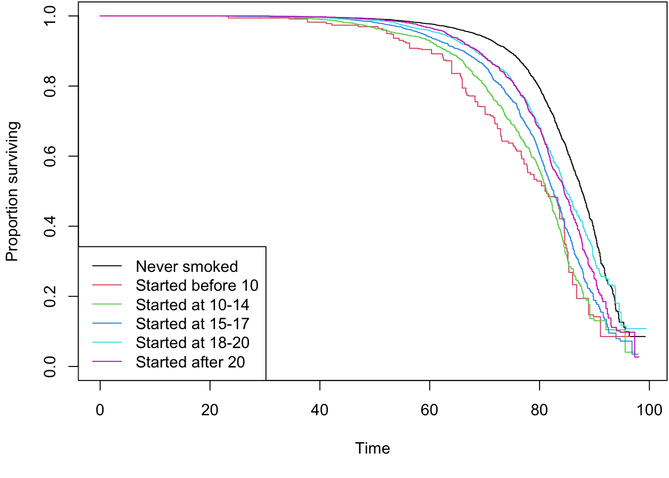
The following code generates a survey-weighted Kaplan-Meier survival curve to visualize the probability of survival over time, stratified by the age of smoking initiation.

Show/Hide Code

dummy <- length(unique(as.factor(w.design0$variables$exposure.cat)))
formulax0 <- as.formula(Surv(stime.since.birth, status_all) ~ exposure.cat)
sA<-svykm(formulax0, design=w.design0)

# Plot
par(oma=rep(0,4))
par(mar=c(5,4,0,0) + 0.1)
plot(sA, pars=list(col=c(1:dummy)),
     xlab = "Time",
     ylab = "Proportion surviving")
legend("bottomleft", levels(as.factor(w.design0$variables$exposure.cat)),
       col = (1:dummy), lty = c(1,1))

Sensitivity Analysis 1: Survey-Weighted Kaplan-Meier Curves

Log-Rank Test

The following code performs a weighted log-rank test to see if the differences between the curves are statistically significant.

Show/Hide Code

# Weighted logrank test
lrt <- svylogrank(formulax0,design=subset(w.design0, survey.weight.new>0))
round(lrt[[2]],2)
#>  Chisq      p 
#> 271.25   0.00

Cox Proportional Hazards Models

The following code fits several survey-weighted Cox models to estimate the Hazard Ratios (HRs) for all-cause mortality associated with smoking initiation age. We fit:

1. An unadjusted (crude) model.
1. An adjusted model, controlling for sex, race, survey year, and the SES proxy variables (pir and HHedu).
1. Two effect modification models to see if the association is different across racial/ethnic groups and by sex.

Show/Hide Code

# Test One
fit0_ <- coxph(Surv(stime.since.birth, status_all) ~ exposure.cat, data = dat.complete)
fit0_


# Unadjusted model
fit0 <- svycoxph(Surv(stime.since.birth, status_all) ~ exposure.cat, 
                 design = w.design0)
fit0

# Adjusted model overall with SES proxies as covariates
fit1 <- svycoxph(Surv(stime.since.birth, status_all) ~ exposure.cat + sex + race + year.cat + pir + HHedu,
                 design = w.design0)
fit1

# Effect modification by race model + proxies
fit2 <- svycoxph(Surv(stime.since.birth, status_all) ~ exposure.cat*race
                 + sex  + year.cat + pir +HHedu,
                 design = w.design0)
fit2

# Effect modification by sex model + proxies
fit3 <- svycoxph(Surv(stime.since.birth, status_all) ~ exposure.cat*sex 
                 + race + year.cat + pir + HHedu,
                 design = w.design0)
fit3

R Code Chunk 8: Prepare Data for Forest Plot

The following code extracts the Hazard Ratios and 95% Confidence Intervals from each of the four models above: fit0, fit1, fit2, and fit3. It then combines them into a single data frame (fr) that will be used to create a summary forest plot.

Show/Hide Code

# Extract results from crude model (fit0)
f0 <- publish(fit0)
f0r <- f0$regressionTable[2:6,c("HazardRatio","CI.95")]
f0r$group <- "Crude"

# Extract results from adjusted model (fit1)
f1 <- publish(fit1)
f1r <- f1$regressionTable[2:6,c("HazardRatio","CI.95")]
f1r$group <- "Adjusted"

# Extract results from race interaction model (fit2)
f2 <- publish(fit2)
f2rW <- f2$regressionTable[(31:35)+8,c("HazardRatio","CI.95")]
f2rB <- f2$regressionTable[(36:40)+8,c("HazardRatio","CI.95")]
f2rH <- f2$regressionTable[(41:45)+8,c("HazardRatio","CI.95")]
f2rW$group <- "White"
f2rB$group <- "Black"
f2rH$group <- "Hispanic"
f2r <- rbind(f2rW, f2rB, f2rH)

# Extract results from sex interaction model (fit3)
f3 <- publish(fit3)
f3rM <- f3$regressionTable[29:33,c("HazardRatio","CI.95")]
f3rF <- f3$regressionTable[34:38,c("HazardRatio","CI.95")]
f3rM$group <- "Male"
f3rF$group <- "Female"
f3r <- rbind(f3rM, f3rF)

# Combine all results into one data frame
fr <- rbind(f0r,f1r,f2r,f3r)
fr <- as.data.frame(fr)
fr$age.grp <- c('Started before 10', 'Started at 10-14', "Started at 15-17",
                "Started at 18-20", "Started after 20")

# Clean up numeric columns
ci <- stringr::str_extract_all(fr$CI.95, '\\d+([.,]\\d+)?', simplify = TRUE)
fr$mean <- as.numeric(fr$HazardRatio)
fr$lower <- as.numeric(as.character(ci[,1]))
fr$upper <- as.numeric(as.character(ci[,2]))
#fr$CI.95 <- NULL
fr$HazardRatio <- NULL

# Save the plot data
frS <- fr
save(frS, file = "data/SensForest.RData")

12.1.3 Visualizing the SES-Adjusted Results

R Code Chunk 9: Plot

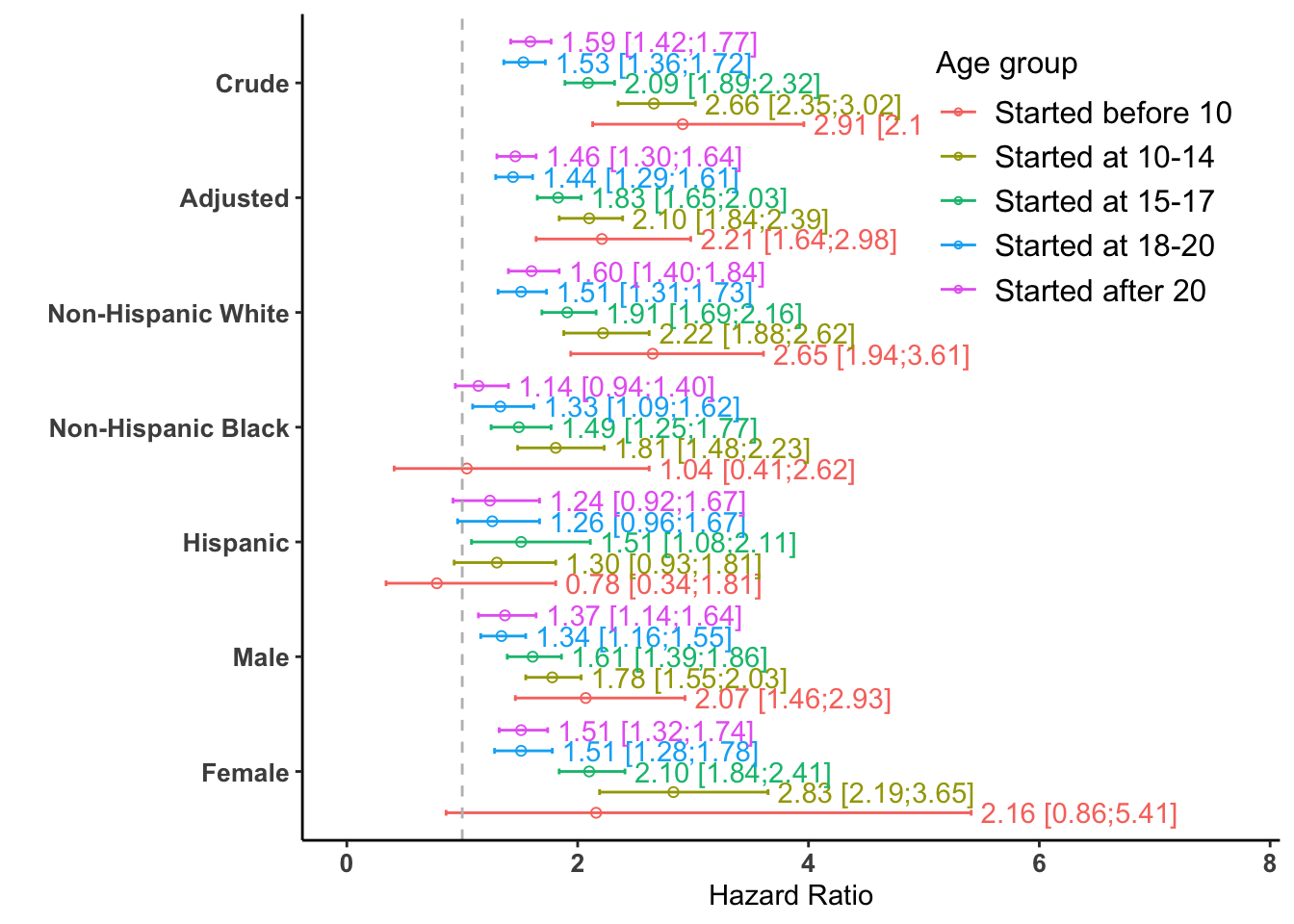
The following code creates the forest plot using ggplot2. The first plot summarizes all the results from this sensitivity analysis. This plot corresponds to Appendix Figure 5 in section C.2 Sensitivity analysis with proxy covariates, part of the supplementary materials published with the paper.

Show/Hide Code

fr$age.grp <- factor(fr$age.grp,
                     levels = c('Started before 10', 'Started at 10-14',
                                "Started at 15-17", "Started at 18-20",
                                "Started after 20"))
fr$group <- factor(fr$group,
                   levels = rev(c("Crude", "Adjusted", 
                                  "White", "Black", "Hispanic", 
                                  "Male", "Female")))
levels(fr$group)[levels(fr$group) == "White"] <- "Non-Hispanic White"
levels(fr$group)[levels(fr$group) == "Black"] <- "Non-Hispanic Black"
fr$text_label <- sprintf("%.2f [%.2f;%.2f]", fr$mean, fr$lower, fr$upper)

# Plotting
ggplot(fr, aes(x = mean, y = group, colour = age.grp)) + 
  geom_errorbar(aes(xmin = lower, xmax = upper), position = position_dodge(0.9), width = 0.25) +
  geom_point(position = position_dodge(0.9), shape = 1) +
  geom_text(aes(label = text_label, x = upper, hjust = -0.05), position = position_dodge(0.9)) +
  scale_x_continuous(limits = c(0, 7.7)) +
  labs(x = "Hazard Ratio", y = "", legend=TRUE, col = "Age group") +
  theme_classic() +
  theme(panel.grid.major.x = element_blank(),
        panel.border = element_blank(),
        legend.title = element_text(size=12), 
        legend.text = element_text(size=12),
        plot.title = element_text(hjust = 0.5),
        axis.text.x = element_text(size = 10, face = "bold"),
        axis.text.y = element_text(size = 10, face = "bold"),
        legend.position = c(.8, .8))+
  geom_vline(xintercept = 1, linetype = "dashed", color = "grey")+
  guides(color = guide_legend(override.aes = list(shape = 1, linetype = 1, size = 1)))
#> Warning: A numeric `legend.position` argument in `theme()` was deprecated in ggplot2
#> 3.5.0.
#> ℹ Please use the `legend.position.inside` argument of `theme()` instead.

Appendix Figure 5: Forest plot of Hazard Ratios from the SES-adjusted sensitivity analysis.

Show/Hide Code

# Save Plot
ggsave("images/forestSens.png", width = 10, height = 8)

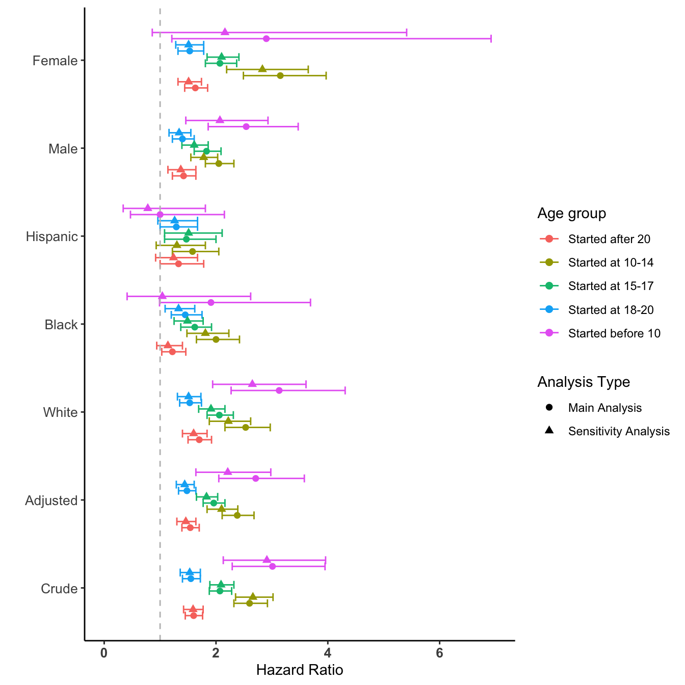
This second plot creates a direct visual comparison between the main analysis results and this sensitivity analysis.

Show/Hide Code

# Load the data for both plots
load(file="data/SensForest.RData")
load(file="data/MainForest.RData")

# Combine data from fr (main) and frS (sensitivity), with an indicator variable
combined_data <- bind_rows(
  mutate(fr, dataset = 'Main Analysis'),
  mutate(frS, dataset = 'Sensitivity Analysis')
)
combined_data$group <- factor(combined_data$group, levels = unique(combined_data$group))

# Create the plot
ggplot(combined_data, aes(x = mean, y = group, colour = age.grp, shape = dataset)) +
  geom_errorbar(aes(xmin = lower, xmax = upper), position = position_dodge(width = 0.7)) +
  geom_point(position = position_dodge(width = 0.7), size = 2) +
  scale_x_continuous(limits = c(0, 7)) +
  labs(x = "Hazard Ratio", y = "", colour = "Age group", shape = "Analysis Type") +
  theme_classic() +
  theme(axis.text.x = element_text(size = 10, face = "bold"),
        axis.text.y = element_text(size = 10),
        legend.position = "right") +
  geom_vline(xintercept = 1, linetype = "dashed", color = "grey")

Comparison of results: Main vs. SES-adjusted Sensitivity Analysis.

Show/Hide Code

# Save Plot
ggsave("images/combined_forest_plot.png", width = 10, height = 6)

12.2 Sensitivity Analysis 2: Effect Modification by Race/Ethnicity (2011-2018)

12.2.1 Data Reprocessing for the 2011-2018 Sub-period

The paper also notes that starting from the 2011−2012 cycle, NHANES introduced a new category labeled non-Hispanic Asian. To investigate the implications of this change, an additional analysis of effect modification by race/ethnicity was conducted specifically for the survey cycles spanning 2011-2018. The following sections re-run similar data merging and cleaning steps, and the different models as in the main analysis code sections, thus only the important changes are noted.

R Code Chunk 1: Redo Data Preparation

The following code shows the respective data needed from the nhanesA library for the 4 cycles and the steps to prepare the specific dataset required for the 2011-2018 sub-period sensitivity analysis. This again, involves downloading raw data, merging them, and constructing necessary variables, mirroring the steps in the main data preparation but for this specific sub-period. The analysis focuses on the 4 cycles spanning 2011-2018.

The same steps are taken, thus only important changes are noted below.

Load Analytic Data for 2011-2018 Cycles and Merge
Load and Merge Mortality Data for Sub-period Analysis
Variable Construction for Sub-period Data
Construct Final Analytic Dataset for Sub-period Analysis
Create Survey Design Object for Sub-period Analysis

Show/Hide Code

# 2011-2012, 2013-2014, 2015-2016, 2017-2018
demo <- c("DEMO_G", "DEMO_H", "DEMO_I", "DEMO_J")
smoking <- c("SMQ_G", "SMQ_H", "SMQ_I", "SMQ_J")

# DEMOGRAPHICS
demo_list_2 <- lapply(demo, nhanes)
demo_data_files <- demo_list_2

# SMOKING
smoking_list_2 <- lapply(smoking, nhanes)
smoking_data_files <- smoking_list_2

The following variables are selected from the data for 4 cycles spanning 2011-2018. The variable RIDRETH3 includes the Race/Hispanic origin w/ NH Asian group. The remaining variables selected are the same as in the main analysis.

Show/Hide Code

demo_columns_2 <- c("SEQN", "RIDAGEYR", "RIAGENDR",
                    "RIDRETH1", "RIDRETH3", "DMDBORN4", 
                    "SDDSRVYR", "WTINT2YR", "WTMEC2YR", 
                    "SDMVPSU", "SDMVSTRA") 

smoking_columns_2 <- c("SEQN", "SMQ020", "SMD030", "SMQ040")

Show/Hide Code

# DEMOGRAPHICS
demo_data_files_2 <- lapply(seq_along(demo_data_files), function(i) 
  {
  current_cycle_data <- demo_data_files[[i]]
  original <- demo[i] 
  
  # Select Columns
  subset_data <- current_cycle_data %>% 
    dplyr::select(dplyr::any_of(demo_columns_2))
  # Translate 
  translated_data <- nhanesTranslate(original,
                                     names(subset_data), 
                                     data = subset_data)
  # Return
  return(translated_data) 
})
#> Translated columns: RIAGENDR RIDRETH1 RIDRETH3 DMDBORN4 SDDSRVYR
#> Translated columns: RIAGENDR RIDRETH1 RIDRETH3 DMDBORN4 SDDSRVYR
#> Translated columns: RIAGENDR RIDRETH1 RIDRETH3 DMDBORN4 SDDSRVYR
#> Translated columns: RIAGENDR RIDRETH1 RIDRETH3 DMDBORN4 SDDSRVYR


# SMOKING
smoking_data_files_2 <- lapply(seq_along(smoking_data_files), function(i) 
  {
  current_cycle_data <- smoking_data_files[[i]]
  original <- smoking[i]

  # Select Columns
  subset_data <- current_cycle_data %>%
    dplyr::select(dplyr::any_of(smoking_columns_2))
  # Translate
  translated_data <- nhanesTranslate(original, 
                                     names(subset_data), 
                                     data = subset_data)
  # Return
  return(translated_data)
})
#> Translated columns: SMQ020 SMQ040
#> Translated columns: SMQ020 SMQ040
#> Translated columns: SMQ020 SMQ040
#> Translated columns: SMQ020 SMQ040


# Merge
data_all <- lapply(seq_along(demo_data_files_2), function(i) {
  demo_df <- demo_data_files_2[[i]]
  smoking_df <- smoking_data_files_2[[i]]
  
  # Merge by SEQN
  merged_df <- join_all(list(demo_df, smoking_df), 
                        by = "SEQN", 
                        type = 'full')
  return(merged_df)
})

R Code Chunk 2: Recode

The following sections of code apply the same recoding except we have another race/ethnicity this time.

ID:

Show/Hide Code

data_all2 <- data_all

# ID
for (i in seq_along(data_all2)) {
  # Set Data
  dat2 <- data_all2[[i]]
  
  # ID
  dat2$id <- dat2$SEQN
  data_all2[[i]] <- dat2
}

Demographic Variables:

Below, the demographic variables like age, sex, and importantly, both race (from RIDRETH1) and race2 (from RIDRETH3 to include Asian) are recoded for the sub-period data.

Show/Hide Code

# Demo
for (i in seq_along(data_all2)) {
  # Set Data
  dat2 <- data_all2[[i]]
  
  # Age
  dat2$age <- dat2$RIDAGEYR
  
  # Sex
  dat2$sex <- dat2$RIAGENDR
  
  # Race/Ethnicity (RIDRETH1 and RIDRETH3)
  dat2$race <- dat2$RIDRETH1
  dat2$race <- car::recode(dat2$race, recodes = "
    'Non-Hispanic White'='White';
    'Non-Hispanic Black'='Black';
    c('Mexican American','Other Hispanic')='Hispanic';
    else='Others'")
  dat2$race <- factor(dat2$race, 
                      levels = c("White", "Black", "Hispanic", "Others"))
  
  
  dat2$race2 <- dat2$RIDRETH3
  dat2$race2 <- car::recode(dat2$race2, recodes = " 
            'Non-Hispanic White'='White';
            'Non-Hispanic Black'='Black'; 
            'Non-Hispanic Asian'='Asian';
            c('Mexican American','Other Hispanic')= 'Hispanic'; 
            else='Others' ")  
  dat2$race2 <- factor(dat2$race2, levels = c("White", "Black",
                                              "Hispanic", "Asian",
                                              "Others"))
  
  
  
  # Country of birth / citizenship
  dat2$born <- dat2$DMDBORN4
  dat2$born <- car::recode(dat2$born, recodes = " 
  'Others'='Other place';
  'Born in 50 US states or Washington, DC'= 'Born in US'; 
  else=NA")
  dat2$born <- factor(dat2$born, 
                      levels = c("Born in US", "Other place"))
  
  data_all2[[i]] <- dat2
  }

Smoking:

Below, the smoking-related variables, including smoking status, age started smoking and whether smoking started at age 15 or younger for the sub-period data are recoded.

Show/Hide Code

# Smoking
for (i in seq_along(data_all2)) {
  # Set Data
  dat2 <- data_all2[[i]]
  
  # Smoking Status
  dat2$smoking <- dat2$SMQ020
  dat2$smoking <- car::recode(dat2$smoking, "
    'Yes' = 'Current smoker';
    'No' = 'Never smoker';
    else = NA")
  dat2$smoking <- factor(dat2$smoking, 
                         levels = c("Never smoker", 
                                    "Previous smoker", 
                                    "Current smoker"))
  
  # Ask about variable SMQ040 ***
  dat2$smoking[dat2$SMQ040 == "Not at all?" | 
                 dat2$SMQ040 == "Not at all"] <- "Previous smoker"
  
  # Age Started Smoking
  dat2$smoking.age <- dat2$SMD030
  dat2$smoking.age[dat2$smoking.age %in% c(777, 999)] <- NA
  dat2$smoking.age[is.na(dat2$smoking.age) & 
                     dat2$smoking == "Never smoker"] <- 0
  
  # Whether Smoking started age ≤ 15
  dat2$smoked.while.child <- car::recode(dat2$smoking.age, 
  " 0 = 'No'; 6:15 = 'Yes'; else = NA ", as.factor = TRUE)
  
  data_all2[[i]] <- dat2
}

Survey Design:

Show/Hide Code

# Survey Design
for (i in seq_along(data_all2)) {
  # Set Data
  dat2 <- data_all2[[i]]
  
  # Weight
  dat2$survey.weight <- dat2$WTINT2YR
  
  # PSU
  dat2$psu <- as.factor(dat2$SDMVPSU)
  
  # Strata
  dat2$strata <- as.factor(dat2$SDMVSTRA)
  
  # Survey year
  dat2$year <- dat2$SDDSRVYR
  
  data_all2[[i]] <- dat2
}

R Code Chunk 3: Save Analytic Data for Sub-period Analysis (Per Cycle)

The following code processes the cleaned sub-period dataframes, applies the age filter (>20 years), selects the final set of variables, and saves them as .RData files for each cycle.

Show/Hide Code


nhanes2_all <- c("nhanes2_11", "nhanes2_13", "nhanes2_15", "nhanes2_17")
vars_2 <- c("id", "age", "sex", "race", "race2", "born", 
          "smoking.age", "smoked.while.child", "smoking", 
          "survey.weight", "psu", "strata", "year")

for (i in seq_along(data_all2)) {
  dat2 <- data_all2[[i]]

  nhanes2_i <- nhanes2_all[i]
  assign(nhanes2_i, dat2[, vars_2], envir = .GlobalEnv)
  
  analytic <- subset(get(nhanes2_i), age >= 20)
  cat("Processing:", nhanes2_i, "\n")
  print(dim(analytic))
  
  analytic_i <- paste0("analytic2_", substr(nhanes2_i, 9, 10))
  analytic_i
  assign(analytic_i, analytic, envir = .GlobalEnv)
  
  # Create 'data' directory if it does not exist
  if (!dir.exists("data")) {
    dir.create("data")
  }
  # Save
  save(list = c(nhanes2_i, analytic_i),
       file = file.path("data", paste0(analytic_i, ".RData")))
  #print(analytic_i)
}
#> Processing: nhanes2_11 
#> [1] 5560   13
#> Processing: nhanes2_13 
#> [1] 5769   13
#> Processing: nhanes2_15 
#> [1] 5719   13
#> Processing: nhanes2_17 
#> [1] 5569   13

R Code Chunk 4: Combine analytic files

The following code ensure the individual analytic .RData files for the sub-period are loaded and combines them into a single dat.full.2 dataframe, recalculating weights for the combined period.

Show/Hide Code

# Load the 4 new datasets
load(file="data/analytic2_11.RData")
load(file="data/analytic2_13.RData")
load(file="data/analytic2_15.RData")
load(file="data/analytic2_17.RData")

# Bind
dat.full.2 <- rbind(nhanes2_11, nhanes2_13, nhanes2_15, nhanes2_17)

# Confirm
unique(dat.full.2$year)
#> [1] NHANES 2011-2012 public release NHANES 2013-2014 public release
#> [3] NHANES 2015-2016 public release NHANES 2017-2018 public release
#> 4 Levels: NHANES 2011-2012 public release ... NHANES 2017-2018 public release
length(unique(dat.full.2$year))
#> [1] 4

# Corrected weights
dat.full.2$survey.weight.new <- dat.full.2$survey.weight/length(unique(dat.full.2$year))
dat.full.2$survey.weight <- NULL
names(dat.full.2)
#>  [1] "id"                 "age"                "sex"               
#>  [4] "race"               "race2"              "born"              
#>  [7] "smoking.age"        "smoked.while.child" "smoking"           
#> [10] "psu"                "strata"             "year"              
#> [13] "survey.weight.new"
dim(dat.full.2)
#> [1] 39156    13

R Code Chunk 5: Load and Merge Mortality Data for Sub-period Analysis

The following code loads the individual mortality datasets for the 4 cycles and combines them. Subsequently, it merges this comprehensive mortality data with the full sub-period analytic dataset (dat.full.2) using the id variable.

Show/Hide Code

mort2000 <- readRDS(file = "data/Mortalitydata/mort2000.RData")
mort2001 <- readRDS(file = "data/Mortalitydata/mort2001.RData")
mort2003 <- readRDS(file = "data/Mortalitydata/mort2003.RData")
mort2005 <- readRDS(file = "data/Mortalitydata/mort2005.RData")
mort2007 <- readRDS(file = "data/Mortalitydata/mort2007.RData")
mort2009 <- readRDS(file = "data/Mortalitydata/mort2009.RData")
mort2011 <- readRDS(file = "data/Mortalitydata/mort2011.RData")
mort2013 <- readRDS(file = "data/Mortalitydata/mort2013.RData")
mort2015 <- readRDS(file = "data/Mortalitydata/mort2015.RData")
mort2017 <- readRDS(file = "data/Mortalitydata/mort2017.RData")

dat.mortality.2 <- rbind(mort2000, mort2001, mort2003,
                       mort2005, mort2007, mort2009, 
                       mort2011, mort2013, mort2015, 
                       mort2017)

dat.full.with.mortality.2 <- merge(dat.full.2, dat.mortality.2, 
                                   by = "id", all.x = TRUE)
dim(dat.full.with.mortality.2)
#> [1] 39156    20

The following code applies recoding which is also similar to main analysis.

Show/Hide Code

dat.full.with.mortality.2$exposure.cat <- car::recode(dat.full.with.mortality.2$smoking.age, " 
                                                    0 = 'Never smoked'; 
                                                    1:9 = 'Started before 10';
                                                    10:14 = 'Started at 10-14';
                                                    15:17 = 'Started at 15-17';
                                                    18:20 = 'Started at 18-20';
                                                    21:80 = 'Started after 20';
                                                    else = NA ", 
                                                    as.factor = TRUE)
dat.full.with.mortality.2$exposure.cat <- factor(dat.full.with.mortality.2$exposure.cat, 
                                               levels = c("Never smoked",
                                                          'Started before 10',
                                                          'Started at 10-14',
                                                          "Started at 15-17",
                                                          "Started at 18-20",
                                                          "Started after 20"))


# Survival time - Person-Months of Follow-up from NHANES Interview date
# changed to "Number of Person Months of Follow-up from NHANES Mobile Examination Center (MEC) date" from "Number of Person Months of Follow-up from NHANES interview date" as we are using MCQ data
dat.full.with.mortality.2$stime.since.interview <- dat.full.with.mortality.2$mort_permth_int # mort_permth_exm 
summary(dat.full.with.mortality.2$stime.since.interview) 
#>    Min. 1st Qu.  Median    Mean 3rd Qu.    Max.    NA's 
#>    1.00   34.00   58.00   58.67   82.00  113.00   15424

# Age in month
dat.full.with.mortality.2$age.month <- dat.full.with.mortality.2$age * 12
summary(dat.full.with.mortality.2$age.month)
#>    Min. 1st Qu.  Median    Mean 3rd Qu.    Max. 
#>     0.0   120.0   336.0   386.9   648.0   960.0

# Survival time - Person-Months of Follow-up from birth = birth to screening + screening to event/censor
dat.full.with.mortality.2$stime.since.birth <- with(dat.full.with.mortality.2, age.month + stime.since.interview)
# converted back to year so that KM plot is in years / HR results remain the same (added)
dat.full.with.mortality.2$stime.since.birth <- dat.full.with.mortality.2$stime.since.birth/12
dat.full.with.mortality.2$stime.since.birth[is.na(dat.full.with.mortality.2$stime.since.interview)] <- NA
summary(dat.full.with.mortality.2$stime.since.birth)
#>    Min. 1st Qu.  Median    Mean 3rd Qu.    Max.    NA's 
#>   19.08   37.17   53.17   53.08   68.17   89.00   15424

# All-cause mortality status
dat.full.with.mortality.2$status_all <- dat.full.with.mortality.2$mort_stat
table(dat.full.with.mortality.2$status_all, useNA = "always")
#> 
#>     0     1  <NA> 
#> 22216  1516 15424

# Cause-specific mortality
dat.full.with.mortality.2$mort_diabetes <- NULL
dat.full.with.mortality.2$mort_hyperten <- NULL
dat.full.with.mortality.2$mort_permth_int <- NULL
dat.full.with.mortality.2$mort_permth_exm <- NULL
dat.full.with.mortality.2$mort_ucod_leading <- NULL
dat.full.with.mortality.2$mort_eligstat <- NULL

R Code Chunk 6: Variable Construction and Final Analytic Dataset for Sub-period Analysis

The same variables are constructed as the main analysis, but note, only for the 4 cycles. Below, the year variable is recoded into categorical levels. Then, the final data set is saved.

Show/Hide Code

# Recode year variable
dat.full.with.mortality.2$year.cat <- dat.full.with.mortality.2$year

new_levels <- c("2011-2012", "2013-2014", "2015-2016", "2017-2018")
levels(dat.full.with.mortality.2$year.cat) <- new_levels

# Display the unique levels of year.cat
levels(dat.full.with.mortality.2$year.cat)
#> [1] "2011-2012" "2013-2014" "2015-2016" "2017-2018"

Show/Hide Code

# Remove variable, not used
dat.full.with.mortality.2$smoked.while.child <- NULL

### Analytic dataset - age 20 - 79
dat.analytic.2 <- subset(dat.full.with.mortality.2, age>=20 & age < 80)
dim(dat.full.with.mortality.2)[1] - dim(dat.analytic.2)[1] # added
#> [1] 18057

# Drop variables that are not being used 
dat.analytic.2$born <- NULL
dat.analytic.2$age <- NULL
dat.analytic.2$age.month <- NULL

# No missing exposure or outcome
dim(dat.analytic.2)
#> [1] 21099    16
dat.analytic1 <- dat.analytic.2[complete.cases(dat.analytic.2$stime.since.birth),]
dim(dat.analytic1)
#> [1] 21011    16
dat.analytic2 <- dat.analytic1[complete.cases(dat.analytic1$exposure.cat),]
dim(dat.analytic2)
#> [1] 20950    16
profile_missing(dat.analytic2)

Profile of missing data after removing participants with missing outcome or exposure. This table confirms that no missing values remain in the key covariates.

Show/Hide Code


# No missing values in covariates - complete case dataset 
dat.complete.2 <- na.omit(dat.analytic2)
dim(dat.complete.2)
#> [1] 20950    16

# Participants dropped - overall
nrow(dat.full.with.mortality.2) - nrow(dat.complete.2)
#> [1] 18206

# Participants dropped - due to missing exposure or outcome
nrow(dat.analytic.2) - nrow(dat.analytic2)
#> [1] 149

# Participants dropped - due to missing covariates
nrow(dat.analytic2) - nrow(dat.complete.2)
#> [1] 0

# added
table(dat.analytic.2$exposure.cat, useNA = "always")
#> 
#>      Never smoked Started before 10  Started at 10-14  Started at 15-17 
#>             12437               126              1497              2769 
#>  Started at 18-20  Started after 20              <NA> 
#>              2440              1767                63

Save the final analytic data for sensitivity analysis used below.

Show/Hide Code

save(dat.complete.2, file = "data/dat.complete.2.RData")

12.2.2 Analysis of the 2011-2018 Sub-period

R Code Chunk 7: Analysis

The following code sets up the survey design object (w.design.2.0) specifically for the 2011-2018 sub-period. It uses the psu, strata, and survey.weight.new variables to correctly account for the complex sampling methodology within this subset of the data. This w.design.2.0 object is essential for running survey-weighted models in this sensitivity analysis.

The following code sets up the survey design object for the 2011-2018 sub-period as in the main analysis.

Show/Hide Code

# Set up the design 
dat.full.with.mortality.2$miss <- 1
dat.full.with.mortality.2$miss[dat.full.with.mortality.2$id %in% dat.analytic2$id] <- 0
table(dat.full.with.mortality.2$miss)
#> 
#>     0     1 
#> 20950 18206

w.design.2 <- svydesign(ids = ~psu, strata = ~strata, weights = ~survey.weight.new, 
                      data = dat.full.with.mortality.2, nest = TRUE)

# Subset the design
w.design.2.0 <- subset(w.design.2, miss == 0 & survey.weight.new > 0)

R Code Chunk 8: Descriptive Statistics for Sub-period (Appendix Table 3)

The following table reproduces Appendix Table 3 from the paper. It summarizes the demographic characteristics of the cohort from the 2011-2018 NHANES cycles, stratified by smoking initiation categories, to provide context for this sensitivity analysis.

Show/Hide Code

# Create the weighted table using the survey design object for the 2011-2018 data
tab_app_3_weighted <- svyCreateTableOne(vars = c("race2"),
                                        strata = "exposure.cat",
                                        data = w.design.2.0,
                                        addOverall = TRUE,
                                        test = TRUE)

# Print and format the table
tab_app_3_printed <- print(tab_app_3_weighted,
                           format = "p",
                           catDigits = 2,
                           showAllLevels = TRUE,
                           smd = TRUE)

# Define the desired column order
new_order_t3 <- c("level", "Never smoked", "Started before 10", 
                  "Started at 10-14", "Started at 15-17", 
                  "Started at 18-20", "Started after 20", 
                  "Overall", "p", "test", "SMD")

# Apply the new order to the table object
tab_app_3 <- tab_app_3_printed[, new_order_t3]

Show/Hide Code

# Display the formatted table using kable for a clean Quarto output
kable(tab_app_3, caption = "Appendix Table 3: Characteristics 
      of the study sample for the 2011-2018 NHANES cycles,
      stratified by smoking initiation age.") %>% 
  kable_styling(bootstrap_options = "striped", full_width = FALSE)

Appendix Table 3: Characteristics of the study sample for the 2011-2018 NHANES cycles, stratified by smoking initiation age.
	level	Never smoked	Started before 10	Started at 10-14	Started at 15-17	Started at 18-20	Started after 20	Overall	p	SMD
n		128386920.10	1240174.76	16008335.09	32086914.62	26126847.18	15892076.56	219741268.30
race2 (%)	White	59.51	74.22	73.86	73.66	68.27	60.61	63.82	<0.001	0.284
	Black	12.39	5.51	7.49	8.55	11.03	16.85	11.59
	Hispanic	17.72	11.12	12.94	11.46	12.77	12.87	15.48
	Asian	7.62	1.33	1.31	2.14	3.40	5.30	5.65
	Others	2.76	7.82	4.40	4.19	4.53	4.36	3.45

Sub-Period Specific Analyses This subsection presents the Kaplan-Meier curve, unadjusted and adjusted Cox models for the 2011-2018 sub-period data, providing initial insights before delving into effect modification.

R Code Chunk 9 : Kaplan-Meier Curves and Log-Rank Test for Sub-period

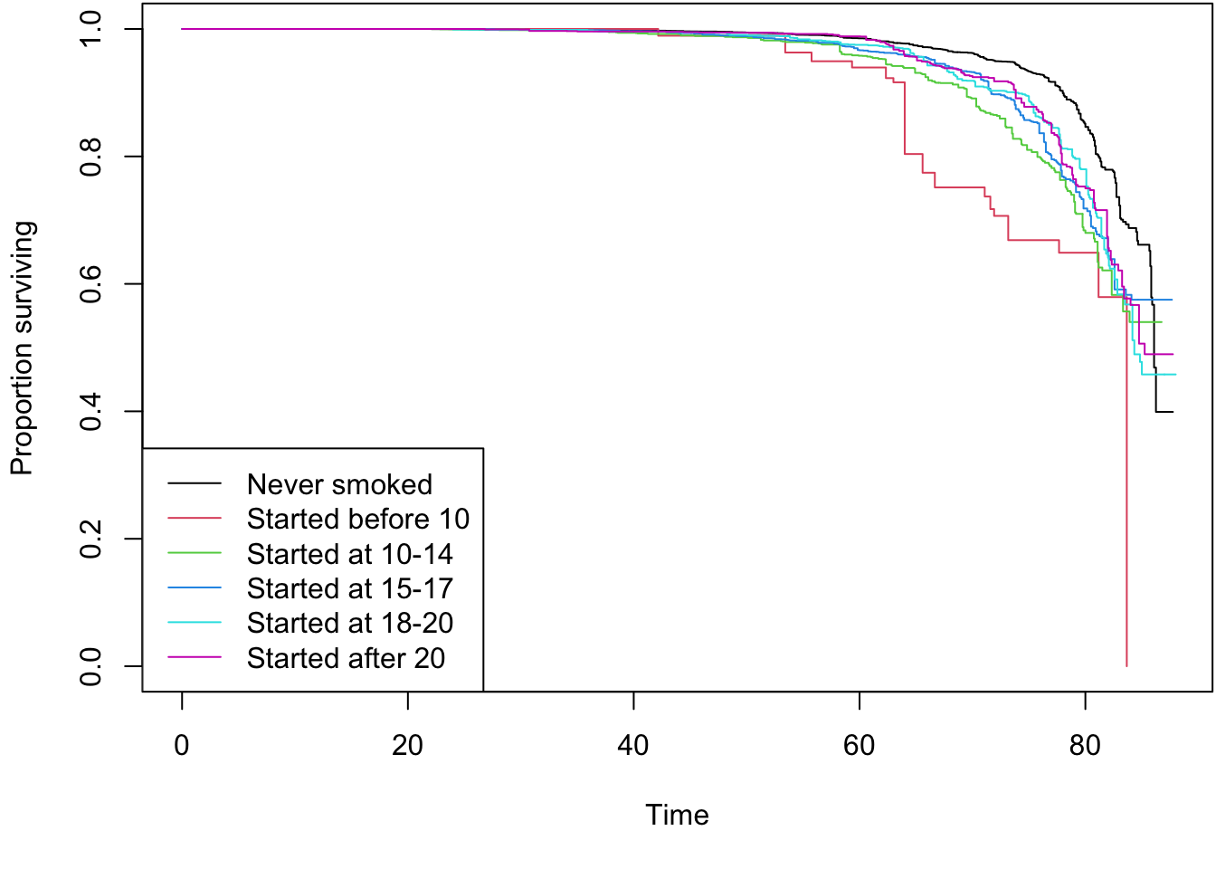
The following code visualizes the survival probabilities for the 2011-2018 sub-period data using Kaplan-Meier curves, stratified by exposure.cat. It also performs a survey-weighted log-rank test to assess statistical differences between the survival curves in this specific subset of the data. The process is the same as the main analysis.

Kaplan-Meier Survival Curves

Show/Hide Code

dummy_sub <- length(unique(as.factor(w.design.2.0$variables$exposure.cat)))

# Define the survival formula for Kaplan-Meier plot and log-rank test
formulax0_sub <- as.formula(Surv(stime.since.birth, status_all) ~ exposure.cat)

# Calculate survey-weighted Kaplan-Meier curves for the sub-period
sA_sub<-svykm(formulax0_sub, design=w.design.2.0)

# Plot
par(oma=rep(0,4))
par(mar=c(5,4,0,0) + 0.1)
plot(sA_sub, pars=list(col=c(1:dummy_sub)),
     xlab = "Time",
     ylab = "Proportion surviving")
legend("bottomleft", levels(as.factor(w.design.2.0$variables$exposure.cat)),
       col = (1:dummy_sub), lty = c(1,1))

Sensitivity Analysis 2: Survey-Weighted Kaplan-Meier Curves

Log-Rank Test

Show/Hide Code

# Perform the survey-weighted log-rank test
lrt_sub <- svylogrank(formulax0_sub,design=subset(w.design.2.0, survey.weight.new>0))
round(lrt_sub[[2]],2)
#> Chisq     p 
#> 40.71  0.00

Cox Proportional Hazards Models

R Code Chunk 10 : Unadjusted Cox Proportional Hazards Models for Sub-period

The following code runs both unweighted (coxph) and survey-weighted (svycoxph) unadjusted Cox proportional hazards models on the sub-period data. These models serve as a baseline for comparison within this specific sensitivity analysis.

Show/Hide Code

# Unweighted Cox model for sub-period
fit0 <- coxph(Surv(stime.since.birth, status_all) ~ exposure.cat, 
              data = dat.complete.2) 

# Survey-weighted unadjusted Cox model for sub-period
fit0 <- svycoxph(Surv(stime.since.birth, status_all) ~ exposure.cat, 
                 design = w.design.2.0) # Using w.design.2.0
f0 <- publish(fit0)

# Process unadjusted HRs for sub-period (similar to main analysis f0r)
f0r <- f0$regressionTable[2:6,c("HazardRatio","CI.95")] 
f0r$group <- "Crude (Sub-period)"
ci_f0_sub <- str_extract_all(f0r[,2], '\\d+([.,]\\d+)?', simplify = TRUE)
f0r$CI.l <- as.numeric(as.character(ci_f0_sub[,1]))
f0r$CI.u <- as.numeric(as.character(ci_f0_sub[,2]))
names(f0r) <- c("mean","CI.95","group","lower","upper")
f0r

R Code Chunk 11: Adjusted Cox Proportional Hazards Model for Sub-period

The following code fits the adjusted Cox proportional hazards model for the sub-period data, controlling for sex, race2, and year.cat.

Show/Hide Code

# Survey-weighted adjusted Cox model for sub-period
fit1 <- svycoxph(Surv(stime.since.birth, status_all) ~ exposure.cat + sex + race2 + year.cat,
                 design = w.design.2.0) 
f1 <- publish(fit1)

# Process adjusted HRs for sub-period (similar to main analysis f1r)
f1r <- f1$regressionTable[2:6,c("HazardRatio","CI.95")]
f1r$group <- "Adjusted (Sub-period)"
ci_f1_sub <- str_extract_all(f1r[,2], '\\d+([.,]\\d+)?', simplify = TRUE)
f1r$CI.l <- as.numeric(as.character(ci_f1_sub[,1]))
f1r$CI.u <- as.numeric(as.character(ci_f1_sub[,2]))
names(f1r) <- c("mean","CI.95","group","lower","upper")
f1r

R Code Chunk 12: Effect Modification by Race/Ethnicity in Sub-period (Model)

The following code fits the core model for the sub-period sensitivity analysis: a survey-weighted Cox proportional hazards model with an interaction term between exposure.cat and race2.

Show/Hide Code

# Model
fit2 <- svycoxph(Surv(stime.since.birth, status_all) ~ exposure.cat*race2 + sex  + year.cat,
                           design = w.design.2.0) # Using w.design.2.0
#> Warning in coxph.fit(X, Y, istrat, offset, init, control, weights = weights, :
#> Loglik converged before variable 24 ; coefficient may be infinite.
f2 <- publish(fit2)

# Process Race-Specific Hazard Ratios for Sub-period Plotting
f2rW <- f2$regressionTable[31:35,c("HazardRatio","CI.95")]
f2rB <- f2$regressionTable[36:40,c("HazardRatio","CI.95")]
f2rH <- f2$regressionTable[41:45,c("HazardRatio","CI.95")]
f2rA <- f2$regressionTable[46:50,c("HazardRatio","CI.95")]
# Assign group labels
f2rW$group <- "White (Sub-period)"
f2rB$group <- "Black (Sub-period)"
f2rH$group <- "Hispanic (Sub-period)"
f2rA$group <- "Asian (Sub-period)"
f2r <- rbind(f2rW, f2rB, f2rH, f2rA)
ci <- str_extract_all(f2r[,2], '\\d+([.,]\\d+)?', simplify = TRUE)
f2r$CI.l <- as.numeric(as.character(ci[,1]))
f2r$CI.u <- as.numeric(as.character(ci[,2]))
names(f2r) <- c("mean","CI.95","group","lower","upper")
f2r

R Code Chunk 13: Effect Modification by Sex in Sub-period (Model)

The following code fits a survey-weighted Cox proportional hazards model, including an interaction term between exposure.cat and sex for the sub-period data.

Show/Hide Code

fit3 <- svycoxph(Surv(stime.since.birth, status_all) ~ exposure.cat*sex + race2 + year.cat, # Using fit3
                 design = w.design.2.0) 
f3 <- publish(fit3)

# Process Sex-Specific Hazard Ratios for Sub-period Plotting
f3rM <- f3$regressionTable[16:20,c("HazardRatio","CI.95")]
f3rF <- f3$regressionTable[21:25,c("HazardRatio","CI.95")]

f3rM$group <- "Male (Sub-period)"
f3rF$group <- "Female (Sub-period)"
f3r <- rbind(f3rM, f3rF)
ci <- str_extract_all(f3r[,2], '\\d+([.,]\\d+)?', simplify = TRUE)
f3r$CI.l <- as.numeric(as.character(ci[,1]))
f3r$CI.u <- as.numeric(as.character(ci[,2]))
names(f3r) <- c("mean","CI.95","group","lower","upper")

12.2.3 Visualizing the Sub-period Results

R Code Chunk 14: Plot

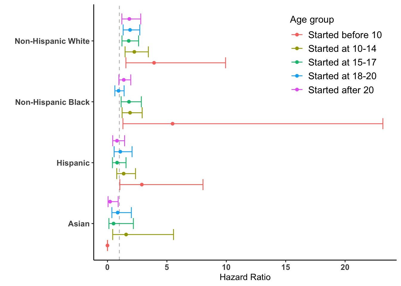
The following code creates the plot using ggplot2 and corresponds to Appendix Figure 4 in section C.1, Sensitivity analysis with ‘Asian’ category, part of the supplementary materials published with the original paper.

Show/Hide Code

fr <- rbind(f2r)
fr <- as.data.frame(fr)
fr[,c(1,4,5)] <- sapply(fr[,c(1,4,5)], as.numeric)
fr$age.grp <- c("Started before 10", "Started at 10-14", "Started at 15-17",
                "Started at 18-20", "Started after 20")
# Change levels
fr$group <- fct_recode(fr$group,
  "Non-Hispanic White" = "White (Sub-period)",
  "Non-Hispanic Black" = "Black (Sub-period)",
  "Hispanic"           = "Hispanic (Sub-period)",
  "Asian"              = "Asian (Sub-period)"
)

# Re-order
fr$age.grp <- factor(fr$age.grp,
                     levels = c("Started before 10",
                                "Started at 10-14",
                                "Started at 15-17",
                                "Started at 18-20",
                                "Started after 20"))

fr$group <- factor(fr$group, levels = c("Asian", "Hispanic", 
                                        "Non-Hispanic Black", "Non-Hispanic White"))

# Plot
ggplot(fr, aes(x = mean, y = group, colour = age.grp)) + 
  geom_vline(xintercept = 1, linetype = "dashed", color = "grey") +
  geom_errorbar(aes(xmax = lower, xmin = upper), position = "dodge") + 
  geom_point(position = position_dodge(0.9)) + 
  labs(x = "Hazard Ratio", y = "", 
       legend=TRUE, col = "Age group") +
  theme_classic() +
  theme(panel.grid.major.x = element_blank(),
        panel.border = element_blank(),
        legend.title=element_text(size=12), 
        legend.text=element_text(size=12),
        plot.title = element_text(hjust = 0),
        axis.text.x = element_text(size = 10, face = "bold"),
        axis.text.y = element_text(size = 10, face = "bold"),
        legend.position=c(.8, .8))

Appendix Figure 4: Forest plot of Hazard Ratios from the sensitivity analysis with ‘Asian’ category.

Show/Hide Code

ggsave("images/forest2.png")
#> Saving 7 x 5 in image

This concludes the sensitivity analysis.

12.3 Appendix B: Exploratory Analysis of Smoking Duration

As noted in the main paper, the duration of smoking is a potential mediator in the pathway from early smoking initiation to mortality. To investigate this secondary relationship, we create boxplots to visualize smoking duration across the different age-of-initiation categories. The following analysis uses the data we set aside earlier (dat.analytic.duration.analysis). This analysis reproduces Appendix Figures 1, 2, and 3 from the paper.

NOTE: This analysis is based on participants from 1999-2016, as the variable for age of smoking cessation (SMD055) was not collected in the 2017-2018 cycle.

12.3.1 Data Preparation for Duration Plots

R Code Chunk 1: Prepare Data for Duration Analysis

The following code processes the data to calculate smoking duration by cleaning the age variables, computing the difference, correcting for data entry errors, and saving the final, plot-ready dataset.

Show/Hide Code

# Clean the 'smoking.age' variable before calculation.
# Recode 0 and 99 (codes for never-smokers) to NA.
dat.analytic.duration.analysis$smoking.age[dat.analytic.duration.analysis$smoking.age == 0] <- NA
dat.analytic.duration.analysis$smoking.age[dat.analytic.duration.analysis$smoking.age == 99] <- NA

# Calculate smoking duration.
dat.analytic.duration.analysis$smoking.duration <- dat.analytic.duration.analysis$smoking.quit.age - dat.analytic.duration.analysis$smoking.age

# Correct any negative durations (from data entry errors) to 0.
dat.analytic.duration.analysis$smoking.duration[!is.na(dat.analytic.duration.analysis$smoking.duration) & dat.analytic.duration.analysis$smoking.duration < 0] <- 0

# Run the original summary checks to explore the new variable.
cat("Total number of participants with non-missing smoking duration data:\n")
#> Total number of participants with non-missing smoking duration data:
print(sum(!is.na(dat.analytic.duration.analysis$smoking.duration)))
#> [1] 8916

cat("\nSummary of smoking duration for all ever-smokers:\n")
#> 
#> Summary of smoking duration for all ever-smokers:
print(summary(dat.analytic.duration.analysis$smoking.duration))
#>    Min. 1st Qu.  Median    Mean 3rd Qu.    Max.    NA's 
#>    0.00    8.00   18.00   19.99   30.00   68.00   41908

# Create the final data frame for plotting by filtering out non-smokers.
dat.analytic.plot <- dat.analytic.duration.analysis %>% 
  filter(!exposure.cat %in% c("Never smoked", NA))

# Save the final plot-ready data.
saveRDS(dat.analytic.plot, file = "data/duration_plot_data.rds")

12.3.2 Visualizing Smoking Duration by Initiation Age

R Code Chunk 2: Smoking Duration Plots

Now, the following code uses the dat.analytic.plot data version to calculate the median smoking duration for each exposure category, which will be used to draw a trend line on the plots.

Show/Hide Code

# Pre-calculate medians for the trend line
median_data <- dat.analytic.plot %>%
  group_by(exposure.cat) %>%
  summarize(median = median(smoking.duration, na.rm = TRUE)) %>%
  arrange(factor(exposure.cat, levels = c('Started before 10',
                                         'Started at 10-14',
                                         "Started at 15-17",
                                         "Started at 18-20",
                                         "Started after 20")))

The following code chunks generate the three plots corresponding to Appendix Figures 1, 2, and 3 in the paper’s supplementary material.

Appendix Figure 1: Overall Smoking Duration

Show/Hide Code

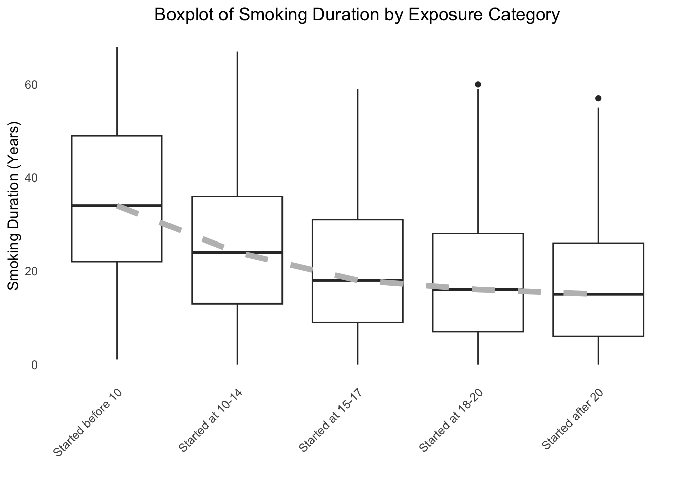
ggplot(dat.analytic.plot, aes(x = exposure.cat, y = smoking.duration, group = exposure.cat)) +
  geom_boxplot(fill = "white") +
  geom_line(data = median_data, aes(x = exposure.cat, y = median, group = 1), color = "grey", size = 2, linetype = 2) +
  geom_smooth(method = "loess", se = TRUE, color = "blue", size = 1, span = 0.5, level = 0.8) +
  theme_minimal() +
  theme(
    legend.position = "none",
    panel.grid.major = element_blank(),
    panel.grid.minor = element_blank(),
    plot.title = element_text(hjust = 0.5),
    axis.text.x = element_text(angle = 45, hjust = 1)
  ) +
  labs(x = "", y = "Smoking Duration (Years)",
       title = "Boxplot of Smoking Duration by Exposure Category")
#> `geom_smooth()` using formula = 'y ~ x'

Smoking duration by age of initiation category among ever-smokers.

Appendix Figure 2: Stratified by Sex

Show/Hide Code

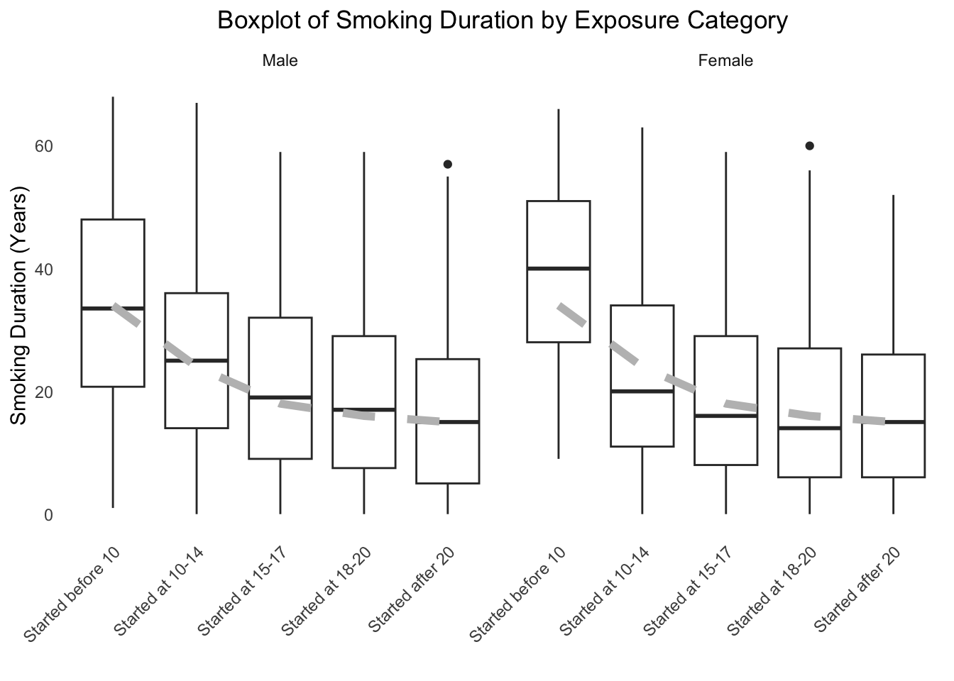
ggplot(dat.analytic.plot, aes(x = exposure.cat, y = smoking.duration, group = exposure.cat)) +
  geom_boxplot(fill = "white") +
  geom_line(data = median_data, aes(x = exposure.cat, y = median, group = 1), color = "grey", size = 2, linetype = 2) +
  geom_smooth(method = "loess", se = TRUE, color = "blue", size = 1, span = 0.5, level = 0.8) +
  facet_wrap(~sex) +
  theme_minimal() +
  theme(
    legend.position = "none",
    panel.grid.major = element_blank(),
    panel.grid.minor = element_blank(),
    plot.title = element_text(hjust = 0.5),
    axis.text.x = element_text(angle = 45, hjust = 1)
  ) +
  labs(x = "", y = "Smoking Duration (Years)",
       title = "Boxplot of Smoking Duration by Exposure Category")
#> `geom_smooth()` using formula = 'y ~ x'

Smoking duration by age of initiation, stratified by sex.

Appendix Figure 3: Stratified by Race/Ethnicity

Show/Hide Code

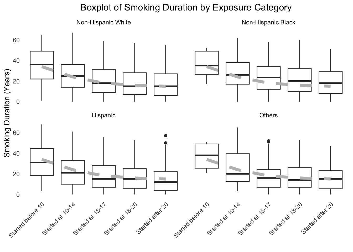
levels(dat.analytic.plot$race)[levels(dat.analytic.plot$race) == "White"] <- "Non-Hispanic White"
levels(dat.analytic.plot$race)[levels(dat.analytic.plot$race) == "Black"] <- "Non-Hispanic Black"

ggplot(dat.analytic.plot, aes(x = exposure.cat, y = smoking.duration, group = exposure.cat)) +
  geom_boxplot(fill = "white") +
  geom_line(data = median_data, aes(x = exposure.cat, y = median, group = 1), color = "grey", size = 2, linetype = 2) +
  geom_smooth(method = "loess", se = TRUE, color = "blue", size = 1, span = 0.5, level = 0.8) +
  facet_wrap(~race) +
  theme_minimal() +
  theme(
    legend.position = "none",
    panel.grid.major = element_blank(),
    panel.grid.minor = element_blank(),
    plot.title = element_text(hjust = 0.5),
    axis.text.x = element_text(angle = 45, hjust = 1)
  ) +
  labs(x = "", y = "Smoking Duration (Years)",
       title = "Boxplot of Smoking Duration by Exposure Category")
#> `geom_smooth()` using formula = 'y ~ x'

Smoking duration by age of initiation, stratified by race/ethnicity.

12.3.3 Interpretation of Results

The boxplots consistently show a clear inverse relationship. The median smoking duration (indicated by the grey dashed line) is highest for those who started smoking before age 10 and steadily decreases for groups that started later in life. This trend holds true when the data is stratified by both sex and race/ethnicity. This visual evidence supports the hypothesis that earlier smoking initiation leads to a longer cumulative exposure to tobacco, which is a likely mediator in the pathway to increased mortality risk.

12.4 Chapter Summary and Next Steps

We have now completed two important sensitivity analyses to test the robustness of our primary findings. First, we adjusted for socioeconomic status proxies, and second, we re-ran the effect modification analysis on the 2011-2018 data to include the non-Hispanic Asian category. The results from both analyses were largely consistent with the main findings, strengthening our confidence in the conclusions.

We also completed the exploratory analysis which suggested a potential mechanism for our findings, showing that earlier smoking initiation is strongly associated with a longer lifetime smoking duration.

With the analytical portion complete, the next chapter, “Discussion of Results,” will synthesize the findings from all analyses and interpret their meaning.