Getting started: one call, eight estimators
Source:vignettes/getting-started.Rmd
getting-started.Rmddr3 implements the average treatment effect (ATE)
estimators reconciled in Three Routes to One Answer. The
organizing idea is that AIPW, TMLE, and double machine learning all
target the same efficient influence function
and differ only in how they solve it (average the
score vs. targeting) and how the nuisances
and
are fit (full-sample, cross-fit, or double cross-fit). dr3
runs the whole family on one shared Super Learner library, so any
difference you see is estimator-driven, not implementation-driven.
One call
We use the canonical Hernán–Robins NHEFS example (quitting smoking →
1971–1982 weight change), which ships in causaldata, so
nothing needs downloading.
d <- dr_nhefs()

# A small library keeps the vignette fast; use default_dr_library for real work.
fit <- dr_panel(d$Y, d$A, d$X, SL.library = c("SL.mean", "SL.glm", "SL.glmnet"),
                seed = 1)
#> Loading required package: nnls
#> Loading required namespace: glmnet
fit
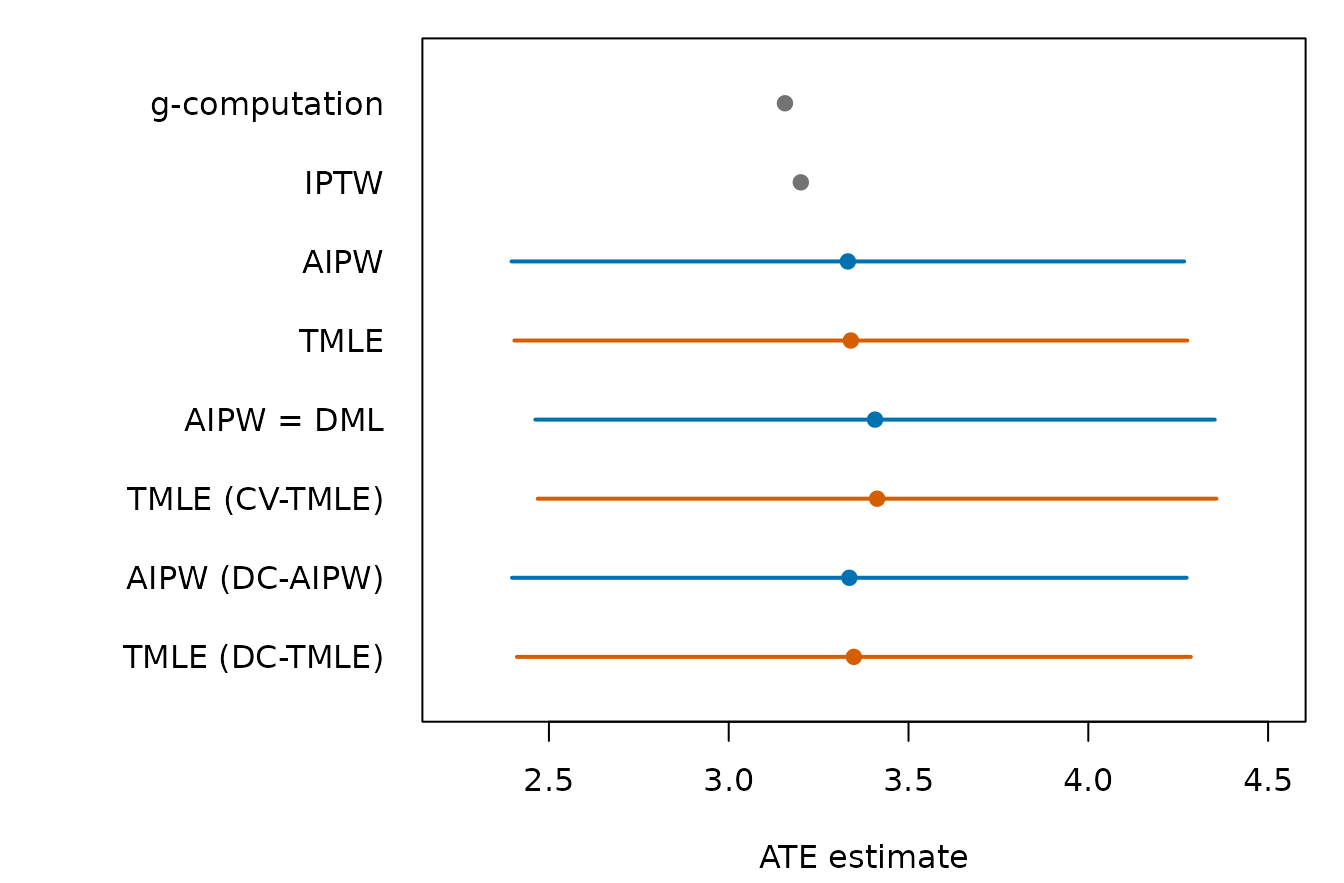
#> dr3 estimator panel  (n = 1566)
#>       estimator         nuisance estimate         95% CI
#>   g-computation             full    3.156
#>            IPTW             full    3.200
#>            AIPW             full    3.331 (2.396, 4.267)
#>            TMLE             full    3.340 (2.404, 4.275)
#>      AIPW = DML        cross-fit    3.407 (2.462, 4.352)
#>  TMLE (CV-TMLE)        cross-fit    3.413 (2.469, 4.356)
#>  AIPW (DC-AIPW) double-cross-fit    3.335 (2.397, 4.274)
#>  TMLE (DC-TMLE) double-cross-fit    3.348 (2.411, 4.285)
The six doubly-robust estimators (AIPW, TMLE, DML, CV-TMLE, DC-AIPW, DC-TMLE) land within about a tenth of a kilogram of one another and of the ~3.4–3.5 kg literature benchmark, while the singly-robust plug-ins (g-computation, IPTW) sit a little apart and carry no analytic interval — exactly the picture the paper draws.
Look under the hood
dr_panel() is a thin wrapper. You can fit the shared
nuisances yourself and hand them to any estimator — pairing
dr_aipw() with cross-fit nuisances is double
machine learning:
nu <- dr_nuisance(d$Y, d$A, d$X, strategy = "crossfit",
                  SL.library = c("SL.mean", "SL.glm", "SL.glmnet"))
dr_aipw(d$Y, d$A, nu)$estimate   # DML
#> [1] 3.406938
dr_tmle(d$Y, d$A, nu)$estimate   # CV-TMLE
#> [1] 3.412667